Lesson 8
NumPy and Numerical Computing
Big question
Why are numerical arrays faster and more expressive than repeatedly updating Python lists?
Lesson progress
Complete checkpoints as you learn
Learning objectives
- Create NumPy arrays.
- Understand shape, dtype, broadcasting, and vectorization.
- Generate reproducible random samples.
- Perform matrix and linear-algebra operations.
- Prerequisites: Chapters 3 to 7.
- Key terms: ndarray, shape, dtype, vectorization, broadcasting, random generator.
Simple explanation
A NumPy array stores values of a common data type in a regular shape. That constraint enables compact memory representation and compiled numerical operations. A one-dimensional array can represent returns; a two-dimensional array can represent observations by variables; higher dimensions appear in images and neural networks. Shape is part of meaning, so analysts should inspect it before matrix multiplication or model fitting (NumPy Developers 2026).
Key terms
- Create NumPy arrays
- A core idea in Chapter 8 that students apply carefully in economic analysis.
- Understand shape, dtype, broadcasting, and vectorization
- A core idea in Chapter 8 that students apply carefully in economic analysis.
- Generate reproducible random samples
- A core idea in Chapter 8 that students apply carefully in economic analysis.
- Perform matrix and linear-algebra operations
- A core idea in Chapter 8 that students apply carefully in economic analysis.
- Prerequisites: Chapters 3 to 7
- A core idea in Chapter 8 that students apply carefully in economic analysis.
- Key terms: ndarray, shape, dtype, vectorization, broadcasting, random generator
- A core idea in Chapter 8 that students apply carefully in economic analysis.
Analytical workflow
Interpret the expression in words and units before using it in a claim.
Example
Interpretation. Each return compares adjacent prices. The output has one fewer observation than the price array.
Prerequisites
- Complete the preceding course chapters or review their summaries as needed.
Full theory and examples
8.2
Arrays are homogeneous numerical structures
A NumPy array stores values of a common data type in a regular shape. That constraint enables compact memory representation and compiled numerical operations. A one-dimensional array can represent returns; a two-dimensional array can represent observations by variables; higher dimensions appear in images and neural networks. Shape is part of meaning, so analysts should inspect it before matrix multiplication or model fitting (NumPy Developers 2026).
8.3
Vectorization states the calculation directly
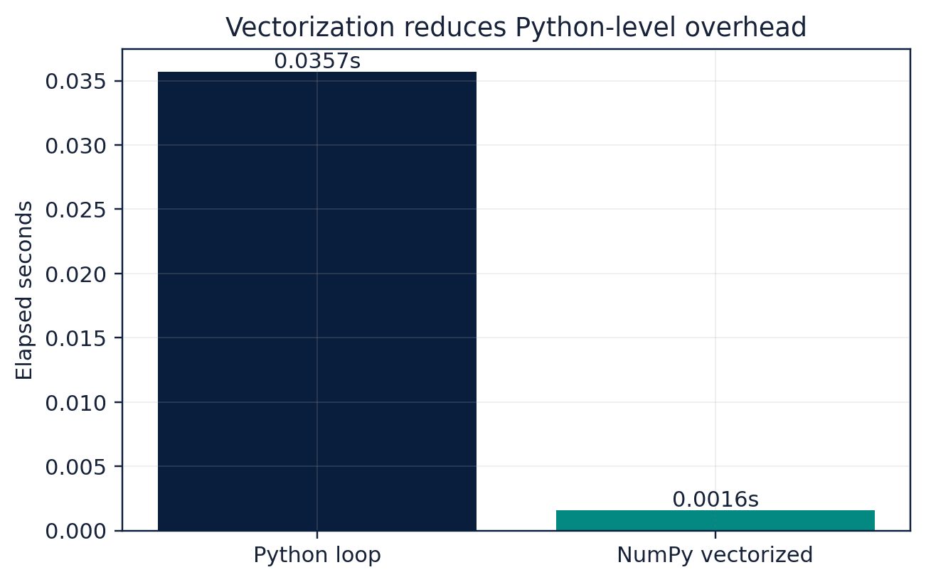
The expression prices[1:] / prices[:-1] - 1 computes a complete return vector without manually managing an index. Vectorization often improves speed because the loop occurs in optimized compiled code. It also exposes the mathematical operation. Broadcasting extends compatible shapes automatically, for example subtracting a column mean from every row. Convenience must be paired with shape checks because an unintended broadcast can produce a plausible but wrong array.
8.4
Randomness should be local and reproducible
Modern NumPy uses a random generator object. Creating rng = np.random.default_rng(seed) keeps the random state explicit and avoids changing a global generator used elsewhere. A seed reproduces a demonstration, not the uncertainty of the real world. Simulation results should still report Monte Carlo error and be checked across additional seeds when conclusions might depend on one stream.
8.5
Core equations
Portfolio return
A weight vector and asset-return vector are combined through a dot product.
8.6
Python demonstrations
8.6.1
Demonstration 8.1: Vectorized return calculation
Verified output
Interpretation. Each return compares adjacent prices. The output has one fewer observation than the price array.
8.6.2
Demonstration 8.2: A reproducible portfolio simulation
Verified output
Interpretation. Matrix multiplication applies the same portfolio weights to every simulated observation.
8.7
Visual evidence
8.8
Reference table
Why This Matters
NumPy is the numerical foundation beneath pandas, statsmodels, scikit-learn, and much of scientific Python.
Common Mistake
Assuming two arrays align because their lengths match. Variables may be in a different order even when the shapes are compatible.
Ceteris LAB Tip
Print shapes at analytical boundaries: after loading, after feature construction, and before model fitting.
R-to-Python / Source Bridge
The source lectures relied on R vectors and matrix operations. NumPy provides the equivalent numerical foundation while making shape and dtype explicit.
| Concept | Question to ask | Typical check |
|---|---|---|
| shape | How many axes and elements? | array.shape |
| dtype | How are values stored? | array.dtype |
| broadcast | Which dimensions are expanded? | compare shapes |
| seed | Can the simulation be repeated? | record generator seed |
Visual evidence
Additional Python demonstrations
Live Python
Source demonstration 2
Source demonstration 2
Stdout
Run Python to see results here.
Status / stderr
Ready to run Python in your browser.
Line-by-line guide
- Line 1Load a Python library needed for data work or regression.
- Line 3Create or update a Python object used in the analysis.
- Line 4Create or update a Python object used in the analysis.
- Line 5Create or update a Python object used in the analysis.
- Line 6Create or update a Python object used in the analysis.
- Line 7Display a result so students can inspect the output.
Verified source output
[ 0.02 -0.0098 0.0297]
[-0.0097 0.004 0.0097 -0.0022 -0.002 ]
[ 0.02 -0.0098 0.0297]
[-0.0097 0.004 0.0097 -0.0022 -0.002 ]
Interpretation. Each return compares adjacent prices. The output has one fewer observation than the price array.
Interpretation. Matrix multiplication applies the same portfolio weights to every simulated observation.
Guided practice
- 1Re-run Demonstration 8.1 and change one input while keeping the analytical question fixed.
- 2Explain in two sentences how the output supports, or fails to support, the chapter opening question.
- 3Add one validation check that would prevent a plausible error.
Exercises
- 1Create a 3 by 2 array and inspect its shape.
- 2Calculate column means and demean the array using broadcasting.
- 3Simulate 1,000 standard-normal values with a generator.
- 4Compute a weighted portfolio return using a dot product.
Source and downloads
Chapter 8 of Fundamentals of Python for Financial Econometrics by Mohammad Safavi, Ph.D.. The lesson is an original Ceteris Lab web adaptation of the supplied publication package.
Live Python
NumPy and Numerical Computing: live Python
NumPy and Numerical Computing: live Python
Stdout
Run Python to see results here.
Status / stderr
Ready to run Python in your browser.
Line-by-line guide
- Line 1Load a Python library needed for data work or regression.
- Line 3Create or update a Python object used in the analysis.
- Line 4Create or update a Python object used in the analysis.
- Line 5Display a result so students can inspect the output.
Python walkthrough
- 1`import numpy as np`: Loads a package or function used by the analysis.
- 2`prices = np.array([100.0, 102.0, 101.0, 104.0])`: Creates or updates a named object used by later steps.
- 3`returns = prices[1:] / prices[:-1] - 1`: Creates or updates a named object used by later steps.
- 4`print(np.round(returns, 4))`: Displays a result so it can be checked and interpreted.
Live notebook
Run this lesson as a notebook
Open an editable notebook cell-by-cell, run Python in the browser, and download the `.ipynb` file for later.
Related dataset
Ceteris Lab teaching sample
Estimated time
25 to 40 min
Packages
pandas, numpy
Expected output
Printed Python results that can be compared with the lesson explanation.
Learning goals
- Load and inspect Ceteris Lab teaching sample.
- Run the Python cells connected to NumPy and Numerical Computing.
- Interpret the output using Create NumPy arrays and Understand shape, dtype, broadcasting, and vectorization.
Common errors
- File not found: check that wage_sample.csv is installed or use the course data folder.
- Package import error: use the browser notebook first, then download for local Jupyter if your local packages differ.
- Column name error: compare your variable names with the dataset variables listed for this notebook.
Dataset path helper
import pandas as pd

df = pd.read_csv("/data/wage_sample.csv")
df.head()
Interactive activity
Chapter 8 interactive
Reproducible Python decision lab
Which step should come before trusting a successful Python run?
Immediate feedback
Choose a decision, then test how the claim changes as evidence becomes stronger or weaker.
Try it yourself
Write one plain-English sentence explaining the main idea from this lesson.
Common mistakes
Check these before you move on.
Return to the lesson assumptions, units, diagnostics, and source evidence to replace this shortcut with a defensible interpretation.
Quick quiz
Which statement best answers the Chapter 8 opening question: Why are numerical arrays faster and more expressive than repeatedly updating Python lists?
Quick quiz
Which practice should be avoided when applying NumPy and Numerical Computing?
Quick quiz
What is the most defensible way to interpret the Python demonstration?
Quick quiz
Why does Chapter 8 matter in an applied econometrics workflow?
Key takeaway
NumPy arrays combine regular shape with efficient numerical operations. Vectorization and broadcasting can clarify mathematical structure. Local random generators improve reproducibility.