Omitted Variables, Measurement Error, Simultaneity, and Endogeneity

This chapter begins from the economic question rather than from software syntax. The goal is to understand what information the data can legitimately provide about omitted variables, measurement error, simultaneity, and endogeneity. Python is used as a transparent laboratory: we state the question, define the target, inspect the data, estimate the model, and then challenge the result.

A recurring distinction in econometrics is the difference between describing a pattern, predicting an outcome, and estimating a causal effect. These goals can use similar equations but require different assumptions. A model may forecast well while offering little causal interpretation, and a credible causal design may deliberately use a simple estimator because identification comes from the research design rather than algorithmic complexity.

Throughout the chapter, pay attention to units, timing, sample construction, and the information set available to the analyst. Economic data are produced by institutions, markets, households, and firms. They are not abstract arrays. A good empirical workflow therefore combines statistical discipline with substantive economic reasoning.

Start with a tiny hypothetical sample that can be checked by hand. Write the unit of observation, outcome, explanatory variable or treatment, and the comparison being made. Before estimating anything, ask what would make the comparison informative and what could make it misleading.

The difference in group averages is easy to compute, but whether it is a causal effect depends on how exposure was assigned and whether the groups are otherwise comparable. This distinction is the heartbeat of modern applied econometrics.

Write the empirical model in a form that makes the target explicit. A generic conditional-mean representation is

E[Y | X] = m(X), or in a linear approximation, Y_i = β₀ + β₁X_i + u_i.

Here Y is the outcome, X denotes observed information, β parameters summarize the chosen model, and u collects other determinants of the outcome. The crucial question is not only whether β can be estimated, but what β means under the design and assumptions.

import numpy as np, statsmodels.api as sm

rng=np.random.default_rng(22)

z=rng.normal(size=400); v=rng.normal(size=400)

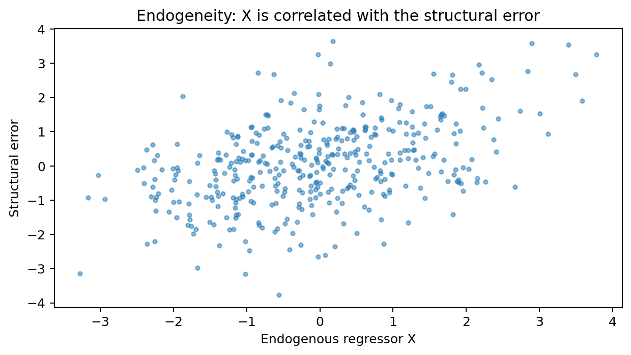
x=.8*z+v; e=.7*v+rng.normal(size=400); y=1+1.5*x+e

print(sm.OLS(y,sm.add_constant(x)).fit().params)

Run the code in a clean notebook and inspect both the numerical output and the data-generating assumptions. The associated notebook in the student package reproduces the example with a fixed random seed.

Figure 22.1. Why can a beautifully estimated regression still answer the wrong question?

Interpret results in the units of the variables. Report sign, magnitude, uncertainty, and the population or time period to which the estimate applies. If a variable is logged, categorical, interacted, standardized, or transformed, translate the coefficient accordingly rather than reading it as a raw one-unit effect.

Then separate statistical significance from economic significance. A precise estimate may be too small to matter economically; an economically important estimate may be imprecise. Both dimensions belong in the conclusion.

Is the unit of observation appropriate for the question?

Are timing and information sets respected?

Could selection, confounding, measurement error, or reverse causality matter?

Does the uncertainty estimator match the sampling or dependence structure?

Would the result survive reasonable alternative specifications?

Is the task predictive, descriptive, or causal?