Lesson 15
Regression and Econometrics with Python
Big question
What does a regression coefficient mean, and which assumptions are needed before it can support an economic claim?
Lesson progress
Complete checkpoints as you learn
Learning objectives
- Estimate simple and multiple linear regressions.
- Interpret coefficients, interactions, and uncertainty.
- Diagnose residual patterns and heteroskedasticity.
- Distinguish explanatory inference from predictive evaluation.
- Prerequisites: Chapters 13 and 14.
- Key terms: OLS, coefficient, residual, robust standard error, interaction, omitted variable.
Simple explanation
Ordinary least squares chooses coefficients that minimize the sum of squared residuals. A slope describes the estimated change in the conditional mean of the outcome associated with a one-unit change in a predictor, holding included variables fixed. That language is descriptive unless the research design supports a causal interpretation. The list of included variables does not by itself eliminate omitted-variable bias.
Key terms
- Estimate simple and multiple linear regressions
- A core idea in Chapter 15 that students apply carefully in economic analysis.
- coefficients, interactions, and uncertainty
- A core idea in Chapter 15 that students apply carefully in economic analysis.
- Diagnose residual patterns and heteroskedasticity
- A core idea in Chapter 15 that students apply carefully in economic analysis.
- explanatory inference from predictive evaluation
- A core idea in Chapter 15 that students apply carefully in economic analysis.
- Prerequisites: Chapters 13 and 14
- A core idea in Chapter 15 that students apply carefully in economic analysis.
- Key terms: OLS, coefficient, residual, robust standard error, interaction, omitted variable
- A core idea in Chapter 15 that students apply carefully in economic analysis.
Analytical workflow
Interpret the expression in words and units before using it in a claim.
Example
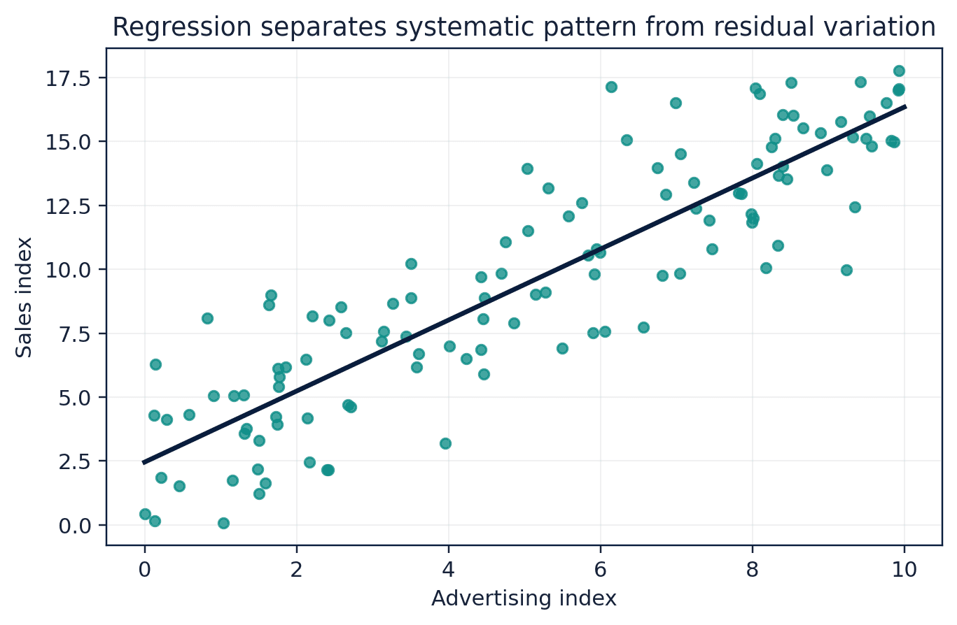
Interpretation. The slope is close to the data-generating value. HC3 standard errors account for heteroskedasticity in a large-sample approximation.
Prerequisites
- Complete the preceding course chapters or review their summaries as needed.
Full theory and examples
15.2
Regression is a conditional comparison
Ordinary least squares chooses coefficients that minimize the sum of squared residuals. A slope describes the estimated change in the conditional mean of the outcome associated with a one-unit change in a predictor, holding included variables fixed. That language is descriptive unless the research design supports a causal interpretation. The list of included variables does not by itself eliminate omitted-variable bias.
15.3
Uncertainty depends on the error structure
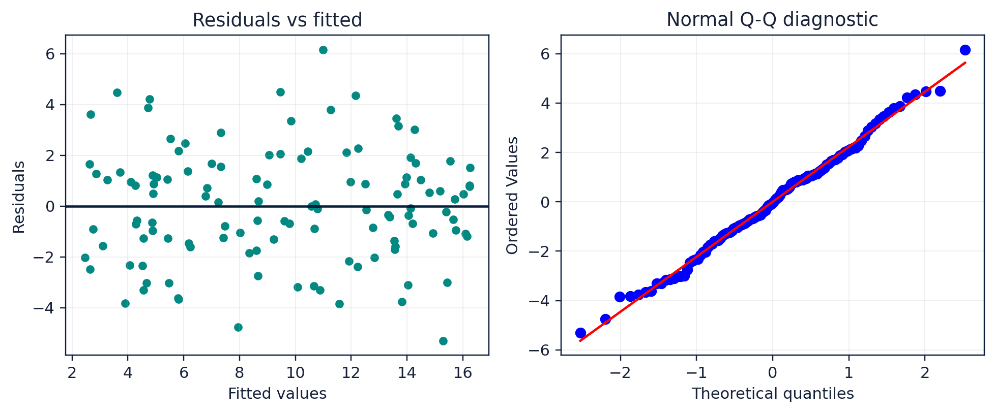
Classical OLS standard errors assume a particular variance and dependence structure. Heteroskedasticity changes the conditional variance across observations; serial or clustered dependence links errors. Robust covariance estimators can improve inference under specified forms of misspecification, but they do not repair biased coefficients or a poorly defined sample. Diagnostics should examine residual plots, leverage, influential observations, and functional form.
15.4
Prediction and inference optimize different questions
statsmodels emphasizes statistical models, coefficient tables, tests, and diagnostics (statsmodels Developers 2026). scikit-learn emphasizes out-of-sample prediction, pipelines, and model comparison (scikit-learn Developers 2026). The same linear formula can serve either purpose, but evaluation differs. A model with interpretable coefficients may not be the best forecaster; a strong predictive model may not identify structural effects.
15.5
Core equations
Linear regression
The residual u captures unobserved components relative to the specified conditional mean.
15.6
Python demonstrations
15.6.1
Demonstration 15.1: Estimate OLS with robust standard errors
Verified output
Interpretation. The slope is close to the data-generating value. HC3 standard errors account for heteroskedasticity in a large-sample approximation.
15.6.2
Demonstration 15.2: Interpret an interaction
Verified output
Interpretation. The interaction allows the slope to differ after x exceeds five. Here the estimated difference is small because the simulated process has one common slope.
15.7
Visual evidence
15.8
Reference table
Why This Matters
Regression provides a disciplined language for conditional relationships, uncertainty, and model diagnostics.
Common Mistake
Describing an observational coefficient as “the impact” without a design that addresses confounding and reverse causality.
Ceteris LAB Tip
Write the coefficient interpretation with units and the phrase “holding included variables fixed” before discussing causality.
R-to-Python / Source Bridge
Regression with serially correlated errors appears later in the source seasonal lecture. This chapter builds the cross-sectional foundation and emphasizes identification before time-series extensions.
| Element | Interpretation | Caution |
|---|---|---|
| coefficient | conditional mean difference | units and coding matter |
| standard error | sampling uncertainty estimate | depends on covariance assumptions |
| R-squared | in-sample variance share | not causality or forecast quality |
| residual | observed minus fitted | not the true structural error |
| interaction | effect depends on another variable | include lower-order terms |
Visual evidence
Additional Python demonstrations
Live Python
Source demonstration 2
Source demonstration 2
Stdout
Run Python to see results here.
Status / stderr
Ready to run Python in your browser.
Line-by-line guide
- Line 1Create or update a Python object used in the analysis.
- Line 2Create or update a Python object used in the analysis.
- Line 3Display a result so students can inspect the output.
Verified source output
0.848 0.028
{'Intercept': 1.503, 'x': 0.809, 'group': -0.565, 'x:group': 0.099}Interpretation. The slope is close to the data-generating value. HC3 standard errors account for heteroskedasticity in a large-sample approximation.
Interpretation. The interaction allows the slope to differ after x exceeds five. Here the estimated difference is small because the simulated process has one common slope.
Guided practice
- 1Re-run Demonstration 15.1 and change one input while keeping the analytical question fixed.
- 2Explain in two sentences how the output supports, or fails to support, the chapter opening question.
- 3Add one validation check that would prevent a plausible error.
Exercises
- 1Estimate a simple regression and interpret the slope.
- 2Add a categorical predictor and explain the reference group.
- 3Compare conventional and HC3 standard errors.
- 4Design a train-test evaluation for a predictive regression.
Source and downloads
Chapter 15 of Fundamentals of Python for Financial Econometrics by Mohammad Safavi, Ph.D.. The lesson is an original Ceteris Lab web adaptation of the supplied publication package.
Live Python
Regression and Econometrics with Python: live Python
Regression and Econometrics with Python: live Python
Stdout
Run Python to see results here.
Status / stderr
Ready to run Python in your browser.
Line-by-line guide
- Line 1Load a Python library needed for data work or regression.
- Line 2Load a Python library needed for data work or regression.
- Line 3Load a Python library needed for data work or regression.
- Line 5Create or update a Python object used in the analysis.
- Line 6Create or update a Python object used in the analysis.
- Line 7Create or update a Python object used in the analysis.
- Line 8Create or update a Python object used in the analysis.
- Line 9Create or update a Python object used in the analysis.
- Line 10Display a result so students can inspect the output.
Python walkthrough
- 1`import numpy as np`: Loads a package or function used by the analysis.
- 2`import pandas as pd`: Loads a package or function used by the analysis.
- 3`import statsmodels.formula.api as smf`: Loads a package or function used by the analysis.
- 4`rng = np.random.default_rng(15)`: Creates or updates a named object used by later steps.
- 5`x = np.linspace(0, 10, 120)`: Creates or updates a named object used by later steps.
- 6`y = 1.5 + 0.8*x + rng.normal(0, 0.4 + 0.08*x)`: Creates or updates a named object used by later steps.
- 7`df = pd.DataFrame({"y": y, "x": x})`: Creates or updates a named object used by later steps.
- 8`model = smf.ols("y ~ x", data=df).fit(cov_type="HC3")`: Fits the specified statistical or machine-learning model.
- 9`print(round(model.params["x"], 3), round(model.bse["x"], 3))`: Displays a result so it can be checked and interpreted.
Live notebook
Run this lesson as a notebook
Open an editable notebook cell-by-cell, run Python in the browser, and download the `.ipynb` file for later.
Related dataset
Ceteris Lab teaching sample
Estimated time
35 to 55 min
Packages
pandas, numpy, matplotlib, statsmodels, patsy
Expected output
A regression or inference table with coefficients, uncertainty, and short interpretation notes.
Learning goals
- Load and inspect Ceteris Lab teaching sample.
- Run the Python cells connected to Regression and Econometrics with Python.
- Interpret the output using Estimate simple and multiple linear regressions and coefficients, interactions, and uncertainty.
Common errors
- File not found: check that wage_sample.csv is installed or use the course data folder.
- Package import error: use the browser notebook first, then download for local Jupyter if your local packages differ.
- Column name error: compare your variable names with the dataset variables listed for this notebook.
Dataset path helper
import pandas as pd

df = pd.read_csv("/data/wage_sample.csv")
df.head()
Interactive activity
Chapter 15 interactive
Data evidence planner
Which choice makes an exploratory result easier to defend?
Immediate feedback
Choose a decision, then test how the claim changes as evidence becomes stronger or weaker.
Try it yourself
Write one plain-English sentence explaining the main idea from this lesson.
Common mistakes
Check these before you move on.
Return to the lesson assumptions, units, diagnostics, and source evidence to replace this shortcut with a defensible interpretation.
Quick quiz
Which statement best answers the Chapter 15 opening question: What does a regression coefficient mean, and which assumptions are needed before it can support an economic claim?
Quick quiz
Which practice should be avoided when applying Regression and Econometrics with Python?
Quick quiz
What is the most defensible way to interpret the Python demonstration?
Quick quiz
Why does Chapter 15 matter in an applied econometrics workflow?
Key takeaway
OLS estimates a conditional linear approximation. Inference depends on covariance assumptions and research design. Explanatory and predictive goals require different evaluation.