Lesson 39
Unit Roots, Seasonality, and Dynamic Regression
Big question
How can a model distinguish persistent trend, recurring seasonality, and serially correlated errors?
Lesson progress
Complete checkpoints as you learn
Learning objectives
- Diagnose unit roots and differencing needs.
- Apply seasonal differencing and decomposition.
- Estimate SARIMA and SARIMAX models.
- Interpret regression with time-series errors cautiously.
- Prerequisites: Chapters 18 and 19.
- Key terms: unit root, seasonality, seasonal difference, SARIMA, SARIMAX, dynamic regression.
Simple explanation
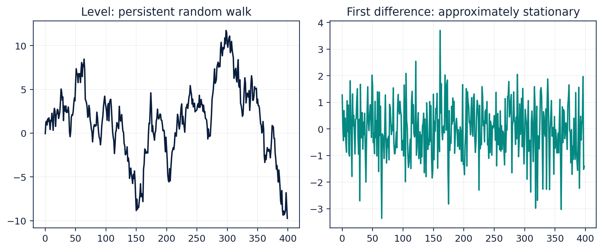
A unit-root process accumulates shocks, so its level does not revert to a fixed mean. First differencing converts a random walk into its innovations. Over-differencing can create unnecessary negative autocorrelation and discard long-run information. ADF results depend on deterministic terms, lag selection, sample length, and structural breaks; the test is evidence rather than a mechanical command.
Key terms
- Diagnose unit roots and differencing needs
- A core idea in Chapter 39 that students apply carefully in economic analysis.
- Apply seasonal differencing and decomposition
- A core idea in Chapter 39 that students apply carefully in economic analysis.
- Estimate SARIMA and SARIMAX models
- A core idea in Chapter 39 that students apply carefully in economic analysis.
- regression with time-series errors cautiously
- A core idea in Chapter 39 that students apply carefully in economic analysis.
- Prerequisites: Chapters 18 and 19
- A core idea in Chapter 39 that students apply carefully in economic analysis.
- Key terms: unit root, seasonality, seasonal difference, SARIMA, SARIMAX, dynamic regression
- A core idea in Chapter 39 that students apply carefully in economic analysis.
Analytical workflow
Interpret the expression in words and units before using it in a claim.
Example
Interpretation. Each month is exactly 12 units above the same month one year earlier in this deterministic illustration.
Prerequisites
- Complete the preceding course chapters or review their summaries as needed.
Full theory and examples
39.2
Differencing removes a stochastic trend, not every trend
A unit-root process accumulates shocks, so its level does not revert to a fixed mean. First differencing converts a random walk into its innovations. Over-differencing can create unnecessary negative autocorrelation and discard long-run information. ADF results depend on deterministic terms, lag selection, sample length, and structural breaks; the test is evidence rather than a mechanical command.
39.3
Seasonality is dependence at a calendar rhythm
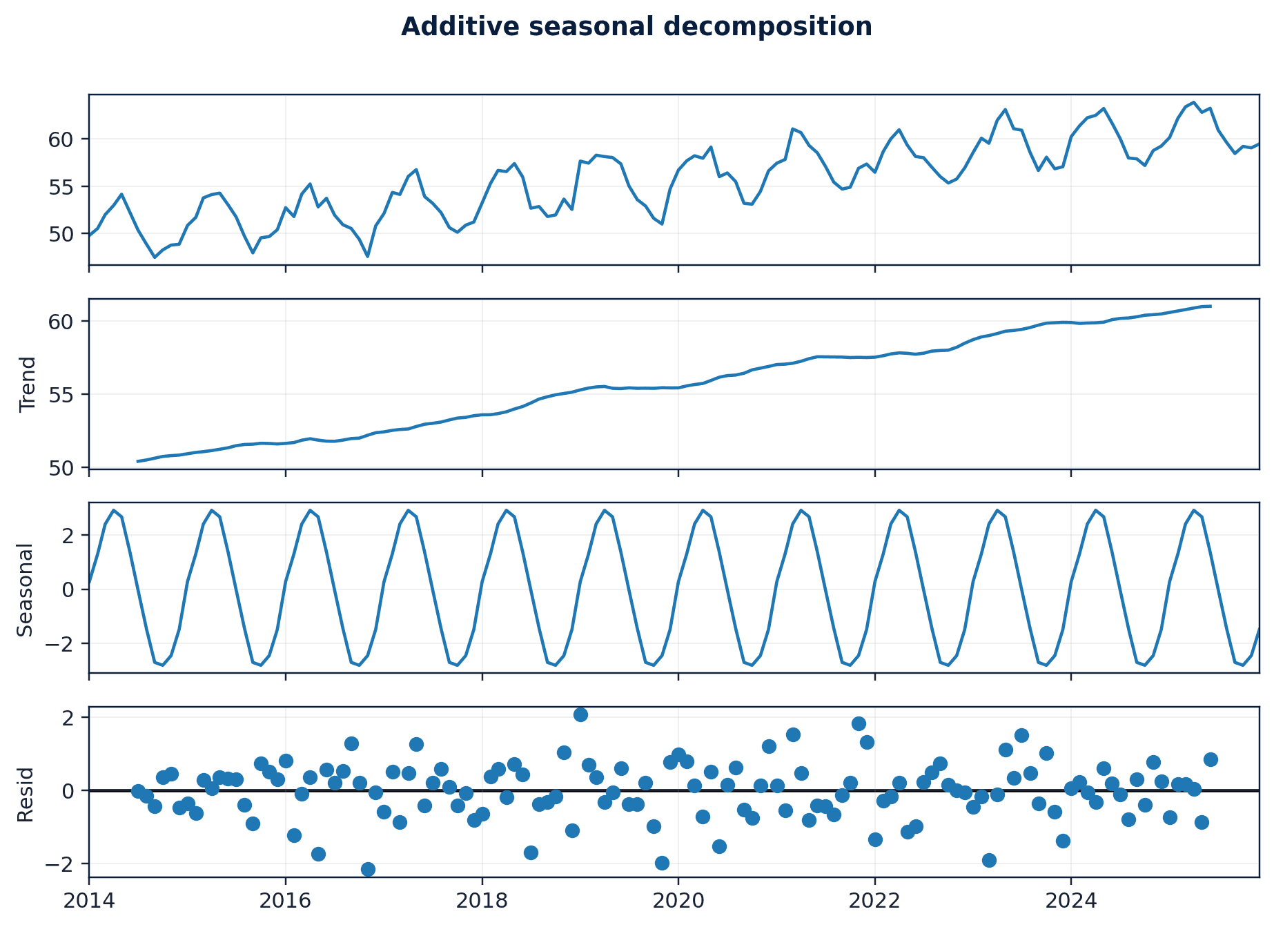
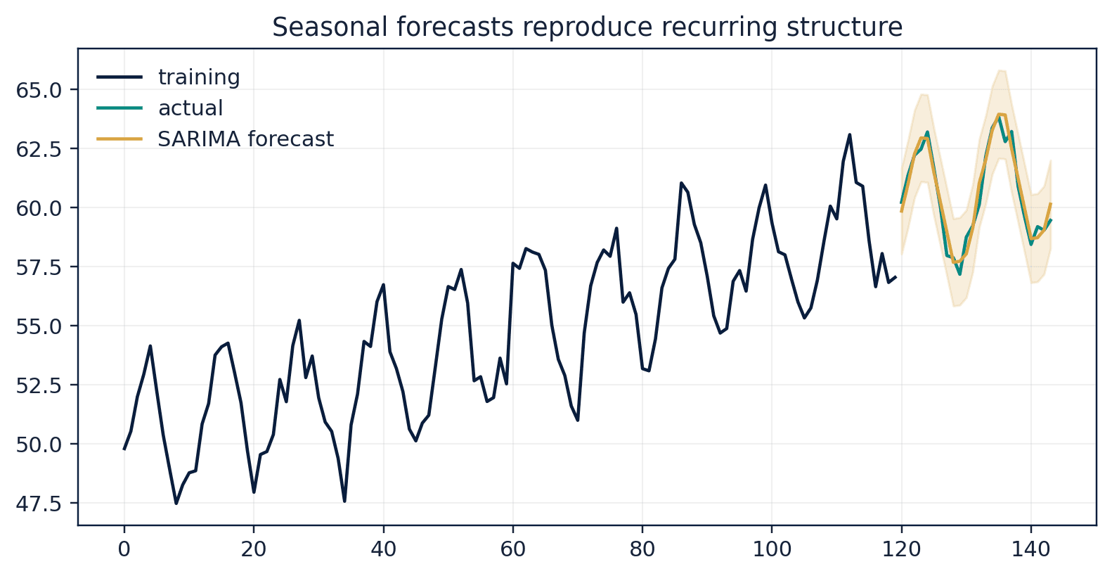
Monthly and quarterly series may repeat patterns because of weather, institutions, holidays, or reporting cycles. Seasonal decomposition separates estimated trend, seasonal, and residual components for exploration. Seasonal differencing compares an observation with the same season in the previous cycle. A multiplicative seasonal ARIMA model allows regular and seasonal AR and MA components to interact.
39.4
Regression errors can remember the past
OLS coefficients remain a conditional linear fit, but serially correlated residuals invalidate ordinary standard-error formulas and signal omitted dynamics. SARIMAX can estimate regression coefficients jointly with ARIMA errors. The regressors must be available at forecast time, and contemporaneous relationships may still be endogenous. A strong fit between two trending series can be spurious unless nonstationarity is addressed.
39.5
Core equations
Seasonal difference
The operator compares the same position in adjacent seasonal cycles.
Airline model
A common regular and seasonal MA specification after regular and seasonal differencing.
39.6
Python demonstrations
39.6.1
Demonstration 20.1: Seasonal differencing
Verified output
Interpretation. Each month is exactly 12 units above the same month one year earlier in this deterministic illustration.
39.6.2
Demonstration 20.2: Fit a seasonal model
Verified output
Interpretation. The exact values depend on the included processed series and estimation conventions. Residual diagnostics remain necessary.
39.7
Visual evidence
39.8
Reference table
Why This Matters
Seasonal and nonstationary structure must be modeled before forecasts or regression standard errors can be trusted.
Common Mistake
Differencing until an ADF p-value crosses a threshold without checking whether the transformed series has an interpretable meaning.
Ceteris LAB Tip
Plot the original, transformed, and seasonally differenced series side by side before selecting a model.
R-to-Python / Source Bridge
The source seasonal lecture covers housing starts, quarterly earnings, the airline model, and regression with serially correlated errors. The new chapter translates those ideas to pandas and SARIMAX while adding benchmark evaluation (Tsay 2013).
| Symptom | Candidate response | Check |
|---|---|---|
| random-walk level | first difference | ADF and forecast performance |
| stable yearly pattern | seasonal difference | seasonal plots and ACF |
| trend plus changing seasonal amplitude | log transform then seasonal model | residual variance |
| serial regression residuals | ARIMA errors/SARIMAX | Ljung-Box residuals |
Visual evidence
Additional Python demonstrations
Live Python
Source demonstration 2
Source demonstration 2
Stdout
Run Python to see results here.
Status / stderr
Ready to run Python in your browser.
Line-by-line guide
- Line 1Load a Python library needed for data work or regression.
- Line 2Load a Python library needed for data work or regression.
- Line 3Load a Python library needed for data work or regression.
- Line 5Create or update a Python object used in the analysis.
- Line 6Create or update a Python object used in the analysis.
- Line 7Create or update a Python object used in the analysis.
- Line 8Run this Python instruction as part of the lesson workflow.
- Line 9Create or update a Python object used in the analysis.
- Line 10Run this Python instruction as part of the lesson workflow.
- Line 11Create or update a Python object used in the analysis.
- Line 12Display a result so students can inspect the output.
- Line 13Display a result so students can inspect the output.
Verified source output
[12.0]
313.71
[61.79, 63.49, 64.73]
313.71 [61.79, 63.49, 64.73]
Interpretation. Each month is exactly 12 units above the same month one year earlier in this deterministic illustration.
Interpretation. The exact values depend on the included processed series and estimation conventions. Residual diagnostics remain necessary.
Guided practice
- 1Re-run Demonstration 20.1 and change one input while keeping the analytical question fixed.
- 2Explain in two sentences how the output supports, or fails to support, the chapter opening question.
- 3Add one validation check that would prevent a plausible error.
Exercises
- 1Simulate a random walk and difference it.
- 2Create monthly seasonal plots.
- 3Fit a seasonal naive benchmark and SARIMA model.
- 4Estimate a regression with AR(1) errors and compare residual diagnostics.
Source and downloads
Chapter 39 of Fundamentals of Python for Financial Econometrics by Mohammad Safavi, Ph.D.. The lesson is an original Ceteris Lab web adaptation of the supplied publication package.
Live Python
Unit Roots, Seasonality, and Dynamic Regression: live Python
Unit Roots, Seasonality, and Dynamic Regression: live Python
Stdout
Run Python to see results here.
Status / stderr
Ready to run Python in your browser.
Line-by-line guide
- Line 1Load a Python library needed for data work or regression.
- Line 3Create or update a Python object used in the analysis.
- Line 4Create or update a Python object used in the analysis.
- Line 5Keep rows that have the variables required for this model.
Python walkthrough
- 1`import pandas as pd`: Loads a package or function used by the analysis.
- 2`series = pd.Series(range(24), index=pd.date_range("2024-01-01", periods=24, freq="MS"))`: Creates or updates a named object used by later steps.
- 3`seasonal_difference = series.diff(12)`: Creates or updates a named object used by later steps.
- 4`print(seasonal_difference.dropna().unique().tolist())`: Displays a result so it can be checked and interpreted.
Live notebook
Run this lesson as a notebook
Open an editable notebook cell-by-cell, run Python in the browser, and download the `.ipynb` file for later.
Related dataset
Ceteris Lab teaching sample
Estimated time
25 to 40 min
Packages
pandas, numpy, statsmodels, patsy
Expected output
A regression or inference table with coefficients, uncertainty, and short interpretation notes.
Learning goals
- Load and inspect Ceteris Lab teaching sample.
- Run the Python cells connected to Unit Roots, Seasonality, and Dynamic Regression.
- Interpret the output using Diagnose unit roots and differencing needs and Apply seasonal differencing and decomposition.
Common errors
- File not found: check that wage_sample.csv is installed or use the course data folder.
- Package import error: use the browser notebook first, then download for local Jupyter if your local packages differ.
- Column name error: compare your variable names with the dataset variables listed for this notebook.
Dataset path helper
import pandas as pd

df = pd.read_csv("/data/wage_sample.csv")
df.head()
Interactive activity
Chapter 39 interactive
Assumption stress test
What should determine the strength of an econometric claim?
Immediate feedback
Choose a decision, then test how the claim changes as evidence becomes stronger or weaker.
Try it yourself
Write one plain-English sentence explaining the main idea from this lesson.
Common mistakes
Check these before you move on.
Return to the lesson assumptions, units, diagnostics, and source evidence to replace this shortcut with a defensible interpretation.
Quick quiz
Which statement best answers the Chapter 39 opening question: How can a model distinguish persistent trend, recurring seasonality, and serially correlated errors?
Quick quiz
Which practice should be avoided when applying Unit Roots, Seasonality, and Dynamic Regression?
Quick quiz
What is the most defensible way to interpret the Python demonstration?
Quick quiz
Why does Chapter 39 matter in an applied econometrics workflow?
Key takeaway
Unit roots create persistent stochastic trends. Seasonal differencing targets recurring calendar dependence. Dynamic regression models coefficients and serial errors jointly.