Lesson 44
Financial Risk Management
Big question
How much could be lost, how often should that threshold be exceeded, and what happens beyond it?
Lesson progress
Complete checkpoints as you learn
Learning objectives
- Define a loss variable and coherent risk principles.
- Calculate VaR and Expected Shortfall.
- Compare historical, parametric, GARCH, and EVT methods.
- Backtest exceedances and discuss stress testing.
- Prerequisites: Chapters 13, 14, 21, and 22.
- Key terms: loss, Value at Risk, Expected Shortfall, backtesting, stress test, extreme-value theory.
Simple explanation
Risk calculations begin by defining a loss variable. For a long position, loss is often negative return times position value; for a short position the sign reverses. VaR is a high quantile of loss over a stated horizon and confidence level. Without the position, horizon, probability, currency, and sign convention, a VaR number is incomplete.
Key terms
- Define a loss variable and coherent risk principles
- A core idea in Chapter 44 that students apply carefully in economic analysis.
- Calculate VaR and Expected Shortfall
- A core idea in Chapter 44 that students apply carefully in economic analysis.
- Compare historical, parametric, GARCH, and EVT methods
- A core idea in Chapter 44 that students apply carefully in economic analysis.
- Backtest exceedances and discuss stress testing
- A core idea in Chapter 44 that students apply carefully in economic analysis.
- Prerequisites: Chapters 13, 14, 21, and 22
- A core idea in Chapter 44 that students apply carefully in economic analysis.
- Key terms: loss, Value at Risk, Expected Shortfall, backtesting, stress test, extreme-value theory
- A core idea in Chapter 44 that students apply carefully in economic analysis.
Analytical workflow
Interpret the expression in words and units before using it in a claim.
Example
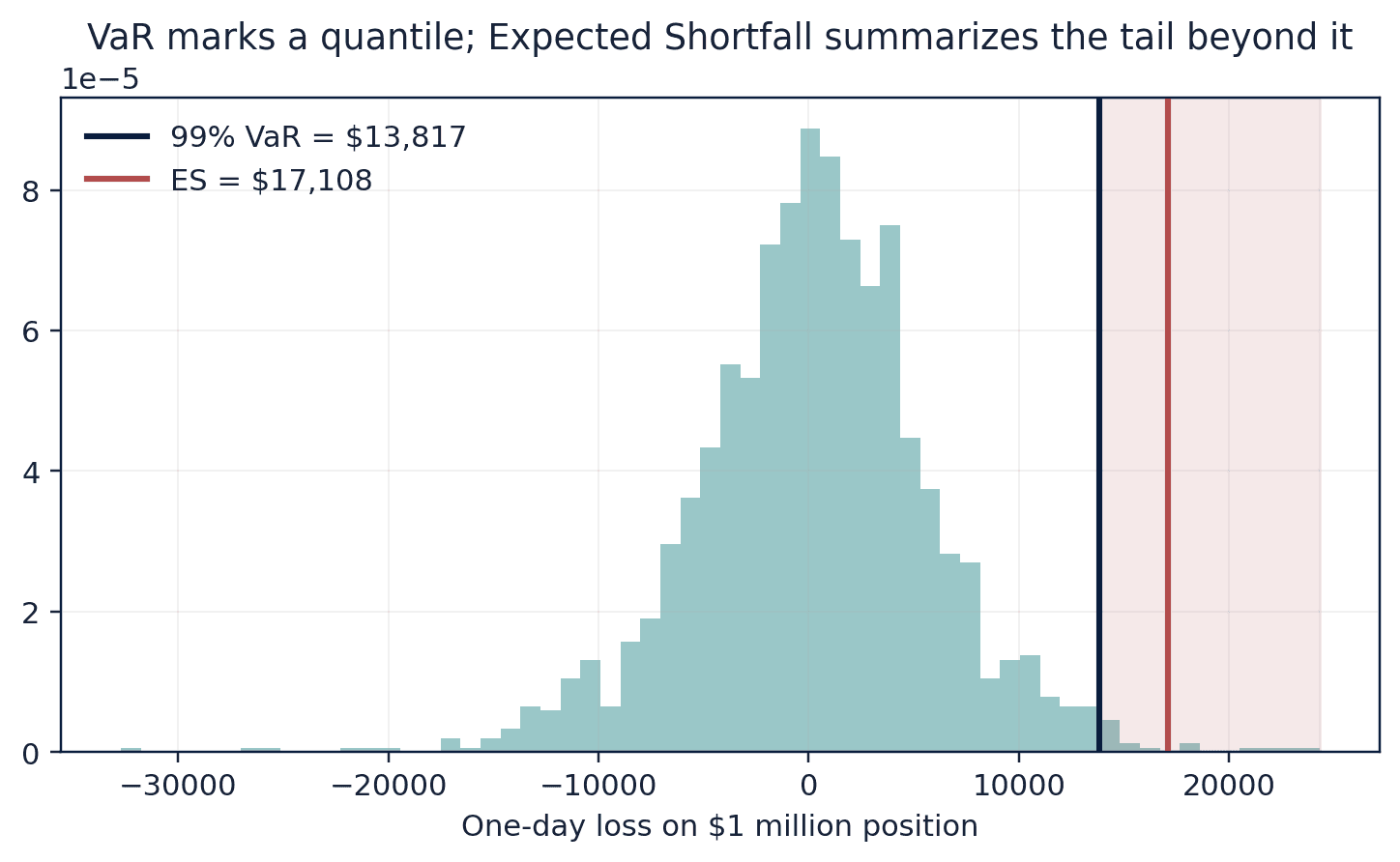
Interpretation. At the 99th percentile, roughly 20 of 2,000 simulated observations lie in the tail used for ES, illustrating tail-sample scarcity.
Prerequisites
- Complete the preceding course chapters or review their summaries as needed.
Full theory and examples
44.2
The sign convention comes first
Risk calculations begin by defining a loss variable. For a long position, loss is often negative return times position value; for a short position the sign reverses. VaR is a high quantile of loss over a stated horizon and confidence level. Without the position, horizon, probability, currency, and sign convention, a VaR number is incomplete.
44.3
Expected Shortfall looks beyond the threshold
VaR identifies a quantile but does not describe the average severity of worse outcomes. Expected Shortfall averages losses in the tail beyond the VaR threshold under a continuous idealization. ES satisfies coherence properties under standard definitions, while VaR can fail subadditivity for some distributions (Artzner et al. 1999). Both remain model-dependent and can be unstable with limited tail data.
44.4
Backtesting checks frequency, not every dimension of risk
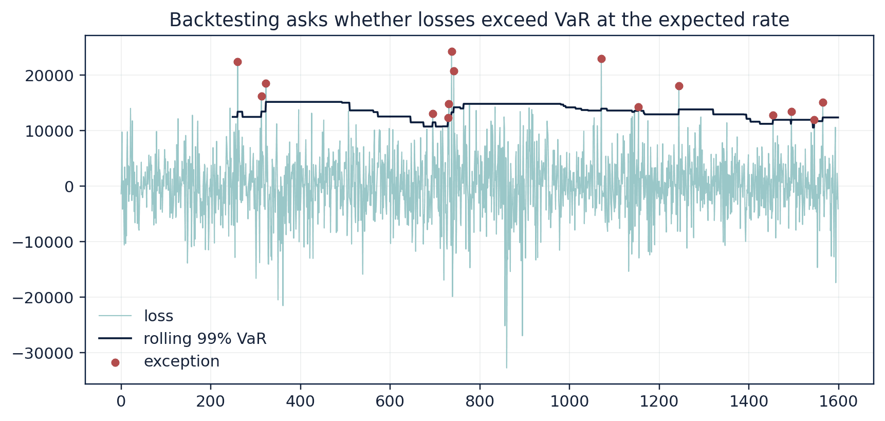
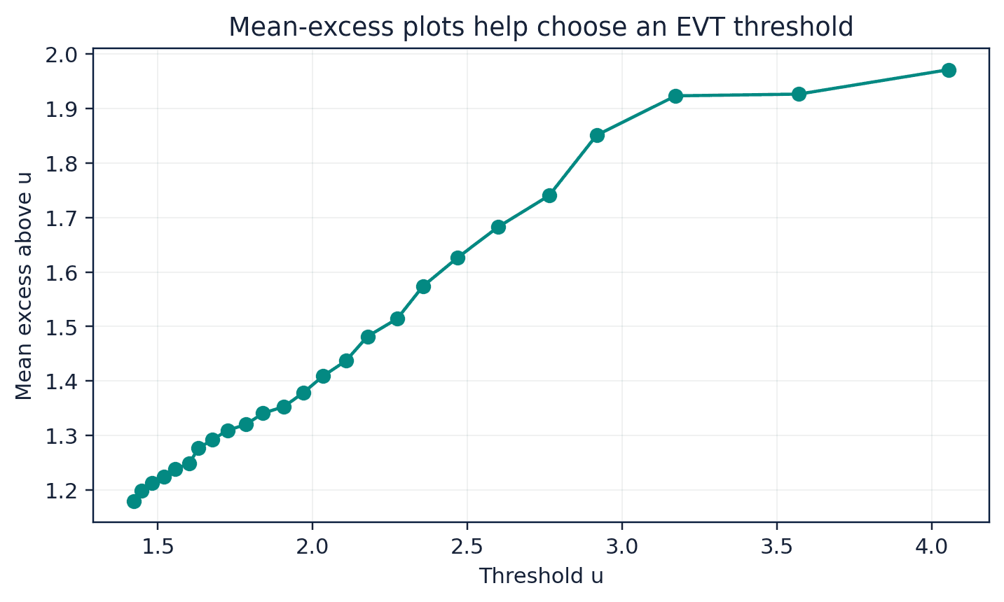
A 99 percent one-day VaR should be exceeded about one percent of the time under a correct conditional model. Too many or too few exceedances indicate calibration problems, while clustered exceedances reveal dependence. Backtests have limited power in short samples and do not validate scenario coverage. Stress testing asks what happens under severe specified conditions, including events absent from the estimation sample. Extreme-value methods focus directly on tail behaviour but introduce threshold and dependence choices.
44.5
Core equations
Value at Risk
The q quantile of the loss distribution.
Expected Shortfall
For a continuous loss distribution, the expected loss beyond VaR.
44.6
Python demonstrations
44.6.1
Demonstration 25.1: Historical VaR and ES
Verified output
Interpretation. At the 99th percentile, roughly 20 of 2,000 simulated observations lie in the tail used for ES, illustrating tail-sample scarcity.
44.6.2
Demonstration 25.2: Count VaR exceedances
Verified output
Interpretation. The unconditional exceedance rate matches by construction for an in-sample historical quantile. A real backtest must forecast each threshold using only prior information.
44.7
Visual evidence
44.8
Reference table
Why This Matters
Risk measures organize a conversation about tail loss, capital, limits, and model uncertainty, but they do not eliminate uncertainty.
Common Mistake
Backtesting a VaR model on the same observations used to estimate each day’s threshold.
Ceteris LAB Tip
Keep losses positive and returns signed in separate variables. This prevents silent sign reversals.
R-to-Python / Source Bridge
The source risk lecture covers coherence, VaR, ES, RiskMetrics, GARCH risk, backtesting, stress testing, and EVT. The Python chapter preserves the mathematical core while strengthening sign, horizon, and out-of-sample controls (Tsay 2013).
| Method | Strength | Weakness |
|---|---|---|
| historical simulation | few distribution assumptions | limited to observed history |
| normal parametric | simple closed form | thin tails and symmetry |
| Student-t parametric | heavier tails | degrees-of-freedom sensitivity |
| GARCH VaR | time-varying volatility | model and innovation risk |
| POT EVT | tail-focused | threshold and dependence sensitivity |
Visual evidence
Additional Python demonstrations
Live Python
Source demonstration 2
Source demonstration 2
Stdout
Run Python to see results here.
Status / stderr
Ready to run Python in your browser.
Line-by-line guide
- Line 1Create or update a Python object used in the analysis.
- Line 2Create or update a Python object used in the analysis.
- Line 3Create or update a Python object used in the analysis.
- Line 4Display a result so students can inspect the output.
Verified source output
0.0383 0.0518 20
20 20.0 0.01
Interpretation. At the 99th percentile, roughly 20 of 2,000 simulated observations lie in the tail used for ES, illustrating tail-sample scarcity.
Interpretation. The unconditional exceedance rate matches by construction for an in-sample historical quantile. A real backtest must forecast each threshold using only prior information.
Guided practice
- 1Re-run Demonstration 25.1 and change one input while keeping the analytical question fixed.
- 2Explain in two sentences how the output supports, or fails to support, the chapter opening question.
- 3Add one validation check that would prevent a plausible error.
Exercises
- 1Compute 95 and 99 percent historical VaR and ES.
- 2Compare normal and Student-t parametric risk.
- 3Design an expanding-window VaR backtest.
- 4Create a stress scenario not present in the historical sample.
Source and downloads
Chapter 44 of Fundamentals of Python for Financial Econometrics by Mohammad Safavi, Ph.D.. The lesson is an original Ceteris Lab web adaptation of the supplied publication package.
Live Python
Financial Risk Management: live Python
Financial Risk Management: live Python
Stdout
Run Python to see results here.
Status / stderr
Ready to run Python in your browser.
Line-by-line guide
- Line 1Load a Python library needed for data work or regression.
- Line 3Create or update a Python object used in the analysis.
- Line 4Create or update a Python object used in the analysis.
- Line 5Create or update a Python object used in the analysis.
- Line 6Create or update a Python object used in the analysis.
- Line 7Create or update a Python object used in the analysis.
- Line 8Create or update a Python object used in the analysis.
- Line 9Display a result so students can inspect the output.
Python walkthrough
- 1`import numpy as np`: Loads a package or function used by the analysis.
- 2`rng = np.random.default_rng(25)`: Creates or updates a named object used by later steps.
- 3`returns = 0.01 * rng.standard_t(df=5, size=2_000)`: Creates or updates a named object used by later steps.
- 4`losses = -returns`: Creates or updates a named object used by later steps.
- 5`q = 0.99`: Creates or updates a named object used by later steps.
- 6`var = np.quantile(losses, q)`: Creates or updates a named object used by later steps.
- 7`es = losses[losses >= var].mean()`: Creates or updates a named object used by later steps.
- 8`print(round(var, 4), round(es, 4), int((losses >= var).sum()))`: Displays a result so it can be checked and interpreted.
Live notebook
Run this lesson as a notebook
Open an editable notebook cell-by-cell, run Python in the browser, and download the `.ipynb` file for later.
Related dataset
Ceteris Lab teaching sample
Estimated time
25 to 40 min
Packages
pandas, numpy
Expected output
Printed Python results that can be compared with the lesson explanation.
Learning goals
- Load and inspect Ceteris Lab teaching sample.
- Run the Python cells connected to Financial Risk Management.
- Interpret the output using Define a loss variable and coherent risk principles and Calculate VaR and Expected Shortfall.
Common errors
- File not found: check that wage_sample.csv is installed or use the course data folder.
- Package import error: use the browser notebook first, then download for local Jupyter if your local packages differ.
- Column name error: compare your variable names with the dataset variables listed for this notebook.
Dataset path helper
import pandas as pd

df = pd.read_csv("/data/wage_sample.csv")
df.head()
Interactive activity
Chapter 44 interactive
Assumption stress test
What should determine the strength of an econometric claim?
Immediate feedback
Choose a decision, then test how the claim changes as evidence becomes stronger or weaker.
Try it yourself
Write one plain-English sentence explaining the main idea from this lesson.
Common mistakes
Check these before you move on.
Return to the lesson assumptions, units, diagnostics, and source evidence to replace this shortcut with a defensible interpretation.
Quick quiz
Which statement best answers the Chapter 44 opening question: How much could be lost, how often should that threshold be exceeded, and what happens beyond it?
Quick quiz
Which practice should be avoided when applying Financial Risk Management?
Quick quiz
What is the most defensible way to interpret the Python demonstration?
Quick quiz
Why does Chapter 44 matter in an applied econometrics workflow?
Key takeaway
VaR is a loss quantile; ES summarizes severity beyond it. Backtesting must use ex ante thresholds. Tail estimation and stress design remain uncertain and model-dependent.