Lesson 37
Dependence, Stationarity, and White Noise
Big question
How can we tell whether a time series contains predictable linear structure rather than random fluctuation?
Lesson progress
Complete checkpoints as you learn
Learning objectives
- Define weak stationarity and white noise.
- Compute and interpret ACF and PACF.
- Apply Ljung-Box and unit-root diagnostics.
- Recognize volatility clustering and nonlinear dependence.
- Prerequisites: Chapter 17 and basic probability.
- Key terms: stationarity, white noise, autocorrelation, partial autocorrelation, Ljung-Box, volatility clustering.
Simple explanation
A weakly stationary series has a constant mean, constant finite variance, and autocovariances that depend on lag rather than calendar date. Stationarity does not mean that every segment looks identical or that shocks are small. It supplies a stable reference for estimating dependence and long-run variance. Prices often appear nonstationary, while returns are closer to stationary, although their conditional variance may still change over time.
Key terms
- Define weak stationarity and white noise
- A core idea in Chapter 37 that students apply carefully in economic analysis.
- Compute and interpret ACF and PACF
- A core idea in Chapter 37 that students apply carefully in economic analysis.
- Apply Ljung-Box and unit-root diagnostics
- A core idea in Chapter 37 that students apply carefully in economic analysis.
- Recognize volatility clustering and nonlinear dependence
- A core idea in Chapter 37 that students apply carefully in economic analysis.
- Prerequisites: Chapter 17 and basic probability
- A core idea in Chapter 37 that students apply carefully in economic analysis.
- Key terms: stationarity, white noise, autocorrelation, partial autocorrelation, Ljung-Box, volatility clustering
- A core idea in Chapter 37 that students apply carefully in economic analysis.
Analytical workflow
Interpret the expression in words and units before using it in a claim.
Example
Interpretation. The simulated white-noise series has small sample autocorrelations and does not reject joint independence at lag 10 in this run.
Prerequisites
- Complete the preceding course chapters or review their summaries as needed.
Full theory and examples
37.2
Stationarity stabilizes the probabilistic frame
A weakly stationary series has a constant mean, constant finite variance, and autocovariances that depend on lag rather than calendar date. Stationarity does not mean that every segment looks identical or that shocks are small. It supplies a stable reference for estimating dependence and long-run variance. Prices often appear nonstationary, while returns are closer to stationary, although their conditional variance may still change over time.
37.3
ACF and PACF are diagnostic fingerprints
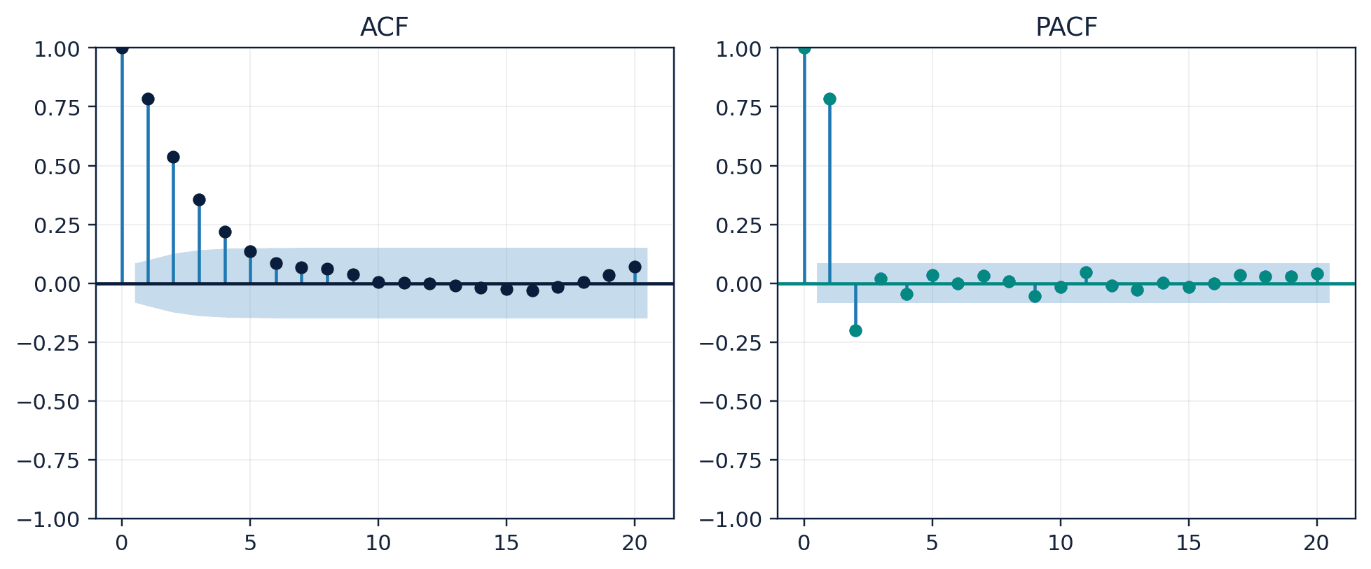
The autocorrelation function measures linear association between observations separated by each lag. The partial autocorrelation removes the linear contribution of shorter lags. Sample values fluctuate even under white noise, so isolated spikes should be interpreted with approximate uncertainty bands and domain context. ACF patterns guide model specification but should not replace estimation and residual checks.
37.4
Uncorrelated does not mean independent
Financial returns may show little autocorrelation while squared or absolute returns show strong persistence. The mean can therefore be difficult to predict even when volatility is predictable. Ljung-Box tests summarize groups of autocorrelations, but p-values depend on lag choice and model estimation. Diagnostics should be applied to raw series, residuals, and transformed residuals according to the model question.
37.5
Core equations
Autocorrelation
For a stationary series, the denominator is constant and dependence is indexed by lag k.
37.6
Python demonstrations
37.6.1
Demonstration 18.1: ACF and Ljung-Box
Verified output
Interpretation. The simulated white-noise series has small sample autocorrelations and does not reject joint independence at lag 10 in this run.
37.6.2
Demonstration 18.2: Levels versus differences
Verified output
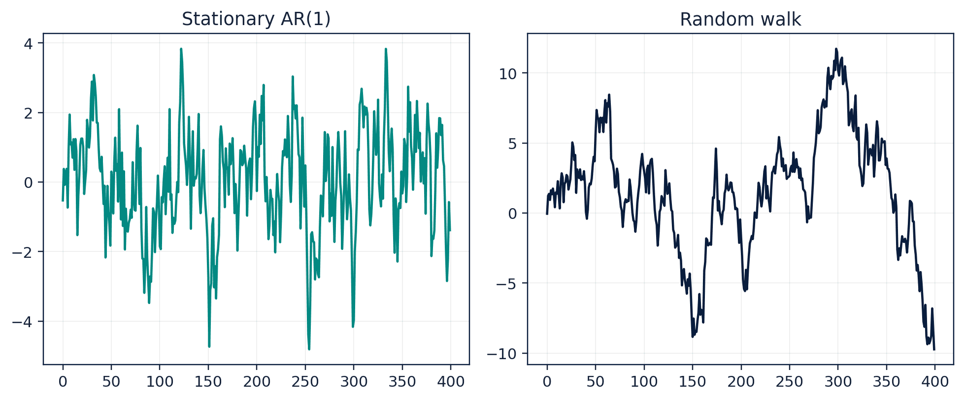
Interpretation. The random-walk level is consistent with a unit root, while its first difference is strongly stationary in the ADF diagnostic.
37.7
Visual evidence
37.8
Reference table
Why This Matters
Dependence diagnostics tell us whether a model has left systematic temporal structure unexplained.
Common Mistake
Calling a series white noise because its mean is near zero. White noise concerns dependence and variance, not only location.
Ceteris LAB Tip
Inspect the ACF of both returns and squared returns before choosing a conditional-mean or volatility model.
R-to-Python / Source Bridge
These concepts are central to the first and second source lectures. The Python version retains the diagnostic sequence while adding explicit distinction between linear and nonlinear dependence (Tsay 2013).
| Diagnostic | Null idea | Use |
|---|---|---|
| ACF | individual lag correlation near zero | pattern discovery |
| PACF | direct lag contribution near zero | AR order guidance |
| Ljung-Box | joint zero autocorrelation through lag m | residual adequacy |
| ADF | unit-root null | nonstationarity diagnostic |
| ACF of squared returns | no linear volatility dependence | ARCH screening |
Visual evidence
Additional Python demonstrations
Live Python
Source demonstration 2
Source demonstration 2
Stdout
Run Python to see results here.
Status / stderr
Ready to run Python in your browser.
Line-by-line guide
- Line 1Load a Python library needed for data work or regression.
- Line 2Load a Python library needed for data work or regression.
- Line 4Create or update a Python object used in the analysis.
- Line 5Create or update a Python object used in the analysis.
- Line 6Create or update a Python object used in the analysis.
- Line 7Display a result so students can inspect the output.
- Line 8Display a result so students can inspect the output.
Verified source output
[1.    0.032 0.046 0.033]
0.844
0.8381
0.00e+00
[1. 0.032 0.046 0.033] 0.844
0.8381 0.00e+00
Interpretation. The simulated white-noise series has small sample autocorrelations and does not reject joint independence at lag 10 in this run.
Interpretation. The random-walk level is consistent with a unit root, while its first difference is strongly stationary in the ADF diagnostic.
Guided practice
- 1Re-run Demonstration 18.1 and change one input while keeping the analytical question fixed.
- 2Explain in two sentences how the output supports, or fails to support, the chapter opening question.
- 3Add one validation check that would prevent a plausible error.
Exercises
- 1Simulate an AR(1) process and compare its ACF with white noise.
- 2Apply Ljung-Box at several lags and discuss multiple testing.
- 3Compare ADF results for a random walk and its difference.
- 4Explain why zero return autocorrelation does not imply independent returns.
Source and downloads
Chapter 37 of Fundamentals of Python for Financial Econometrics by Mohammad Safavi, Ph.D.. The lesson is an original Ceteris Lab web adaptation of the supplied publication package.
Live Python
Dependence, Stationarity, and White Noise: live Python
Dependence, Stationarity, and White Noise: live Python
Stdout
Run Python to see results here.
Status / stderr
Ready to run Python in your browser.
Line-by-line guide
- Line 1Load a Python library needed for data work or regression.
- Line 2Load a Python library needed for data work or regression.
- Line 3Load a Python library needed for data work or regression.
- Line 5Create or update a Python object used in the analysis.
- Line 6Create or update a Python object used in the analysis.
- Line 7Display a result so students can inspect the output.
- Line 8Display a result so students can inspect the output.
Python walkthrough
- 1`import numpy as np`: Loads a package or function used by the analysis.
- 2`from statsmodels.stats.diagnostic import acorr_ljungbox`: Loads a package or function used by the analysis.
- 3`from statsmodels.tsa.stattools import acf`: Loads a package or function used by the analysis.
- 4`rng = np.random.default_rng(18)`: Creates or updates a named object used by later steps.
- 5`x = rng.normal(size=500)`: Creates or updates a named object used by later steps.
- 6`print(np.round(acf(x, nlags=3, fft=True), 3))`: Displays a result so it can be checked and interpreted.
- 7`print(round(acorr_ljungbox(x, lags=[10], return_df=True)["lb_pvalue"].iloc[0], 3))`: Displays a result so it can be checked and interpreted.
Live notebook
Run this lesson as a notebook
Open an editable notebook cell-by-cell, run Python in the browser, and download the `.ipynb` file for later.
Related dataset
Ceteris Lab teaching sample
Estimated time
25 to 40 min
Packages
pandas, numpy
Expected output
Printed Python results that can be compared with the lesson explanation.
Learning goals
- Load and inspect Ceteris Lab teaching sample.
- Run the Python cells connected to Dependence, Stationarity, and White Noise.
- Interpret the output using Define weak stationarity and white noise and Compute and interpret ACF and PACF.
Common errors
- File not found: check that wage_sample.csv is installed or use the course data folder.
- Package import error: use the browser notebook first, then download for local Jupyter if your local packages differ.
- Column name error: compare your variable names with the dataset variables listed for this notebook.
Dataset path helper
import pandas as pd

df = pd.read_csv("/data/wage_sample.csv")
df.head()
Interactive activity
Chapter 37 interactive
Assumption stress test
What should determine the strength of an econometric claim?
Immediate feedback
Choose a decision, then test how the claim changes as evidence becomes stronger or weaker.
Try it yourself
Write one plain-English sentence explaining the main idea from this lesson.
Common mistakes
Check these before you move on.
Return to the lesson assumptions, units, diagnostics, and source evidence to replace this shortcut with a defensible interpretation.
Quick quiz
Which statement best answers the Chapter 37 opening question: How can we tell whether a time series contains predictable linear structure rather than random fluctuation?
Quick quiz
Which practice should be avoided when applying Dependence, Stationarity, and White Noise?
Quick quiz
What is the most defensible way to interpret the Python demonstration?
Quick quiz
Why does Chapter 37 matter in an applied econometrics workflow?
Key takeaway
Stationarity provides a stable dependence framework. ACF, PACF, and Ljung-Box diagnose linear serial structure. Volatility dependence may remain when return autocorrelation is weak.