Lesson 42
Nonlinear Models, Regimes, Market Microstructure, and Ordered Outcomes
Big question
What if the same lag has a different effect in calm and stressed regimes, or the observed price change is an ordered category?
Lesson progress
Complete checkpoints as you learn
Learning objectives
- Simulate and interpret threshold autoregression.
- Explain Markov-switching regimes and expected duration.
- Describe market-microstructure effects.
- Estimate and interpret ordered probit probabilities.
- Prerequisites: Chapters 18, 19, and 22.
- Key terms: TAR, regime, Markov switching, bid-ask bounce, ordered probit, threshold.
Simple explanation
A threshold autoregression applies different linear equations depending on a lagged state variable. Each regime may be simple even when the combined process is nonlinear and asymmetric. Regime-specific coefficients can exceed one in magnitude without automatically making the complete process explosive, because switching rules constrain the path. Simulation and stability analysis are essential.
Key terms
- Simulate and interpret threshold autoregression
- A core idea in Chapter 42 that students apply carefully in economic analysis.
- Markov-switching regimes and expected duration
- A core idea in Chapter 42 that students apply carefully in economic analysis.
- market-microstructure effects
- A core idea in Chapter 42 that students apply carefully in economic analysis.
- Estimate and interpret ordered probit probabilities
- A core idea in Chapter 42 that students apply carefully in economic analysis.
- Prerequisites: Chapters 18, 19, and 22
- A core idea in Chapter 42 that students apply carefully in economic analysis.
- Key terms: TAR, regime, Markov switching, bid-ask bounce, ordered probit, threshold
- A core idea in Chapter 42 that students apply carefully in economic analysis.
Analytical workflow
Interpret the expression in words and units before using it in a claim.
Example
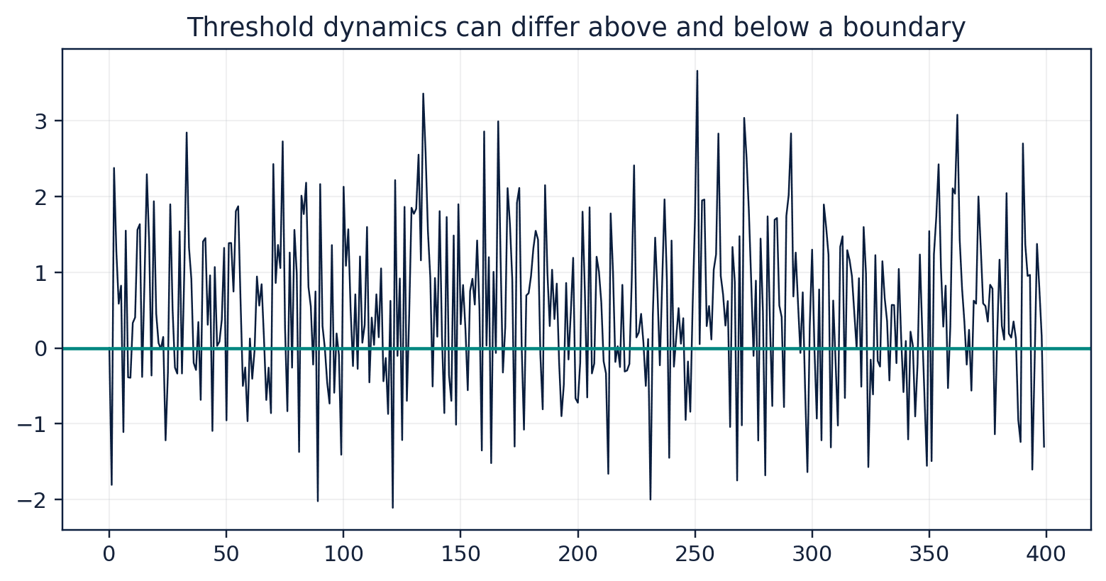
Interpretation. The unconditional mean is positive even though neither regime includes an intercept, illustrating nonlinear asymmetry.
Prerequisites
- Complete the preceding course chapters or review their summaries as needed.
Full theory and examples
42.2
Threshold models make dynamics piecewise
A threshold autoregression applies different linear equations depending on a lagged state variable. Each regime may be simple even when the combined process is nonlinear and asymmetric. Regime-specific coefficients can exceed one in magnitude without automatically making the complete process explosive, because switching rules constrain the path. Simulation and stability analysis are essential.
42.3
Markov switching treats the regime as latent
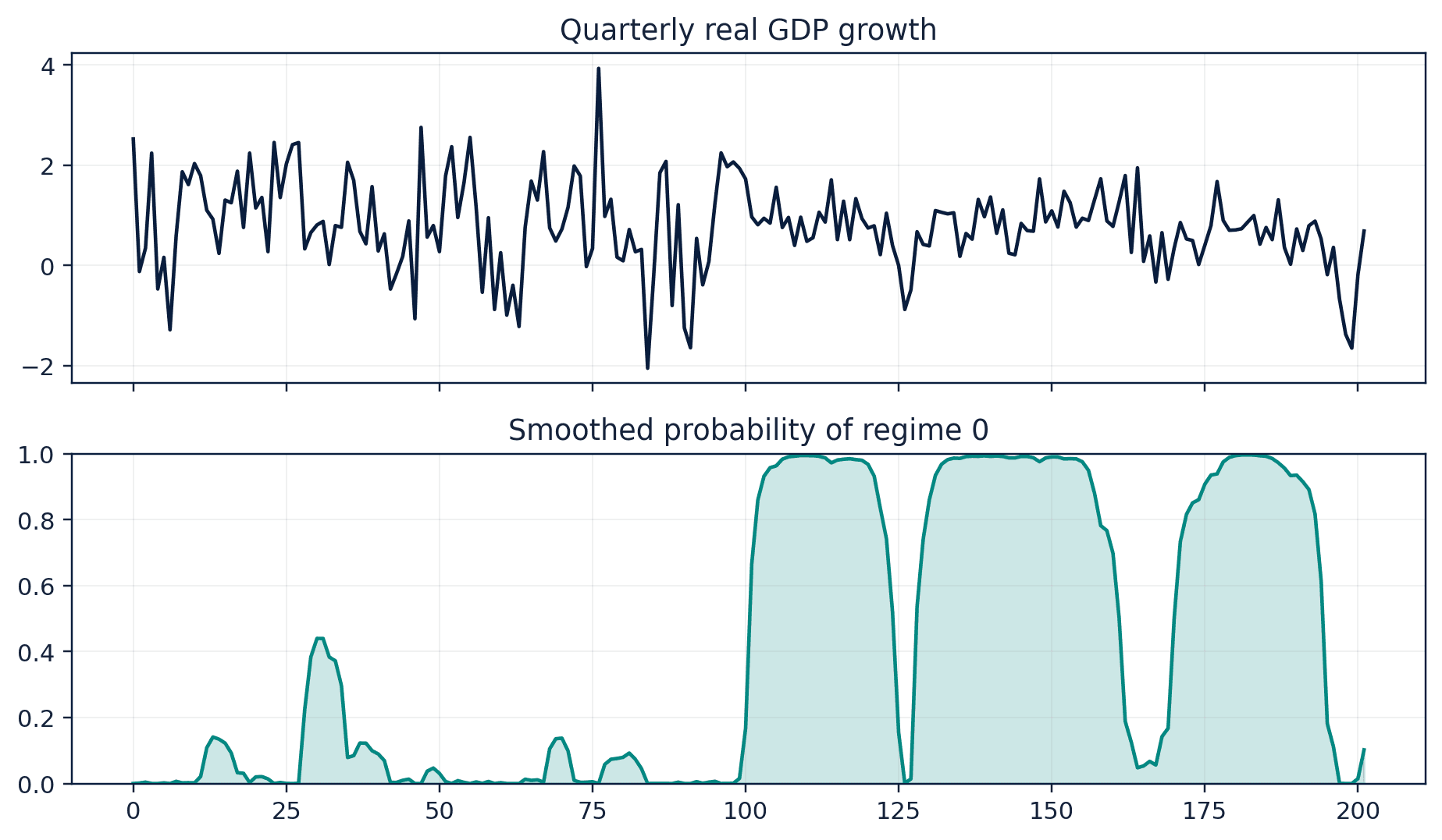
A Markov-switching model assumes an unobserved state that follows transition probabilities. The expected duration of a state is related to the probability of remaining in it. Regime labels are arbitrary and should be interpreted through estimated means, variances, and posterior probabilities. Apparent regimes can also reflect structural breaks or omitted variables rather than a persistent hidden process.
42.4
Market data are generated by trading mechanisms
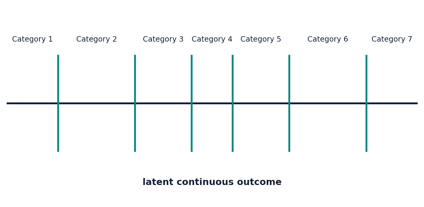
Transaction prices are discrete, trades arrive irregularly, and bid-ask bounce can create negative short-lag dependence. Ordered probit models represent observed categories as intervals of a latent continuous variable. Thresholds and covariates determine category probabilities. The model describes ordering, not equal distance between categories, and a standard implementation assumes a common latent error scale unless extended.
42.5
Core equations
Ordered response
Observed categories arise when a latent index crosses ordered thresholds.
42.6
Python demonstrations
42.6.1
Demonstration 23.1: Simulate a two-regime TAR process
Verified output
Interpretation. The unconditional mean is positive even though neither regime includes an intercept, illustrating nonlinear asymmetry.
42.6.2
Demonstration 23.2: Fit an ordered probit
Verified output
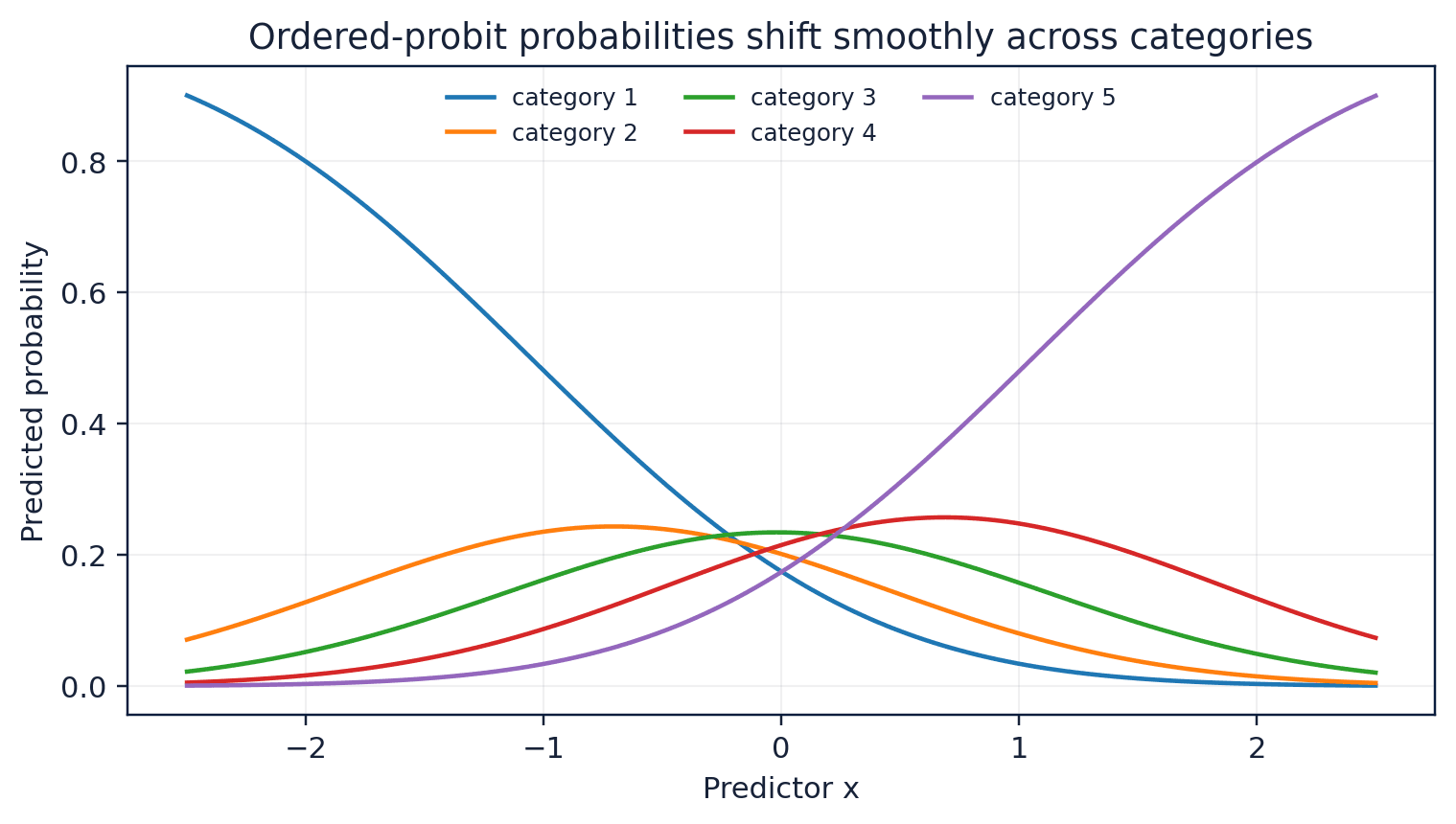
Interpretation. At x=0, the central category is most probable. The probabilities sum to one and depend on both slope and thresholds.
42.7
Visual evidence
42.8
Reference table
Why This Matters
Nonlinear and microstructure models prevent a single linear equation from flattening state-dependent behaviour.
Common Mistake
Interpreting estimated regimes as known historical labels without examining posterior probabilities and uncertainty.
Ceteris LAB Tip
For ordered models, graph predicted category probabilities over a meaningful covariate range instead of reading thresholds in isolation.
R-to-Python / Source Bridge
The source nonlinear lecture and separate ordered-probit handout are integrated here. Python replaces custom R indicators and polr() with transparent feature construction and statsmodels OrderedModel (Tsay 2013).
| Model | State observed? | Key interpretation |
|---|---|---|
| TAR | Yes, threshold variable | piecewise coefficients |
| Markov switching | No | transition probabilities and filtered states |
| ordered probit | Observed category only | latent index and thresholds |
| microstructure model | Trades/quotes observed | institutional price formation |
Visual evidence
Additional Python demonstrations
Live Python
Source demonstration 2
Source demonstration 2
Stdout
Run Python to see results here.
Status / stderr
Ready to run Python in your browser.
Line-by-line guide
- Line 1Load a Python library needed for data work or regression.
- Line 2Load a Python library needed for data work or regression.
- Line 3Load a Python library needed for data work or regression.
- Line 5Create or update a Python object used in the analysis.
- Line 6Create or update a Python object used in the analysis.
- Line 7Create or update a Python object used in the analysis.
- Line 8Create or update a Python object used in the analysis.
- Line 9Create or update a Python object used in the analysis.
- Line 10Display a result so students can inspect the output.
- Line 11Display a result so students can inspect the output.
Verified source output
0.726 0.263
0.805
[0.282 0.518 0.2  ]
0.805 [0.282 0.518 0.2 ]
Interpretation. The unconditional mean is positive even though neither regime includes an intercept, illustrating nonlinear asymmetry.
Interpretation. At x=0, the central category is most probable. The probabilities sum to one and depend on both slope and thresholds.
Guided practice
- 1Re-run Demonstration 23.1 and change one input while keeping the analytical question fixed.
- 2Explain in two sentences how the output supports, or fails to support, the chapter opening question.
- 3Add one validation check that would prevent a plausible error.
Exercises
- 1Simulate a TAR process under two threshold rules.
- 2Fit a Markov-switching mean model.
- 3Explain how bid-ask bounce affects short-lag returns.
- 4Plot ordered-probit category probabilities.
Source and downloads
Chapter 42 of Fundamentals of Python for Financial Econometrics by Mohammad Safavi, Ph.D.. The lesson is an original Ceteris Lab web adaptation of the supplied publication package.
Live Python
Nonlinear Models, Regimes, Market Microstructure, and Ordered Outcomes: live Python
Nonlinear Models, Regimes, Market Microstructure, and Ordered Outcomes: live Python
Stdout
Run Python to see results here.
Status / stderr
Ready to run Python in your browser.
Line-by-line guide
- Line 1Load a Python library needed for data work or regression.
- Line 3Create or update a Python object used in the analysis.
- Line 4Create or update a Python object used in the analysis.
- Line 5Run this Python instruction as part of the lesson workflow.
- Line 6Create or update a Python object used in the analysis.
- Line 7Create or update a Python object used in the analysis.
- Line 8Display a result so students can inspect the output.
Python walkthrough
- 1`import numpy as np`: Loads a package or function used by the analysis.
- 2`rng = np.random.default_rng(23)`: Creates or updates a named object used by later steps.
- 3`x = np.zeros(300)`: Creates or updates a named object used by later steps.
- 4`for t in range(1, len(x)):`: Repeats the indented calculation across observations or simulation draws.
- 5`phi = -1.2 if x[t-1] < 0 else 0.55`: Creates or updates a named object used by later steps.
- 6`x[t] = phi*x[t-1] + rng.normal()`: Creates or updates a named object used by later steps.
- 7`print(round(x.mean(), 3), round((x < 0).mean(), 3))`: Displays a result so it can be checked and interpreted.
Live notebook
Run this lesson as a notebook
Open an editable notebook cell-by-cell, run Python in the browser, and download the `.ipynb` file for later.
Related dataset
Ceteris Lab teaching sample
Estimated time
25 to 40 min
Packages
pandas, numpy, statsmodels, patsy
Expected output
A regression or inference table with coefficients, uncertainty, and short interpretation notes.
Learning goals
- Load and inspect Ceteris Lab teaching sample.
- Run the Python cells connected to Nonlinear Models, Regimes, Market Microstructure, and Ordered Outcomes.
- Interpret the output using Simulate and interpret threshold autoregression and Markov-switching regimes and expected duration.
Common errors
- File not found: check that wage_sample.csv is installed or use the course data folder.
- Package import error: use the browser notebook first, then download for local Jupyter if your local packages differ.
- Column name error: compare your variable names with the dataset variables listed for this notebook.
Dataset path helper
import pandas as pd

df = pd.read_csv("/data/wage_sample.csv")
df.head()
Interactive activity
Chapter 42 interactive
Assumption stress test
What should determine the strength of an econometric claim?
Immediate feedback
Choose a decision, then test how the claim changes as evidence becomes stronger or weaker.
Try it yourself
Write one plain-English sentence explaining the main idea from this lesson.
Common mistakes
Check these before you move on.
Return to the lesson assumptions, units, diagnostics, and source evidence to replace this shortcut with a defensible interpretation.
Quick quiz
Which statement best answers the Chapter 42 opening question: What if the same lag has a different effect in calm and stressed regimes, or the observed price change is an ordered category?
Quick quiz
Which practice should be avoided when applying Nonlinear Models, Regimes, Market Microstructure, and Ordered Outcomes?
Quick quiz
What is the most defensible way to interpret the Python demonstration?
Quick quiz
Why does Chapter 42 matter in an applied econometrics workflow?
Key takeaway
Threshold models use observed regime rules; Markov models use latent states. Trading mechanisms can create dependence in transaction data. Ordered probit maps a latent index into ordered categories.