Lesson 49
Neural Networks and Deep Learning for Economic Data
Big question
How does a stack of simple differentiable units learn a nonlinear mapping, and how do we know it has not merely memorized the training sample?
Lesson progress
Complete checkpoints as you learn
Learning objectives
- Explain neurons, activations, layers, and forward passes.
- Describe backpropagation and optimization.
- Train a small PyTorch network.
- Use learning curves, regularization, and validation.
- Prerequisites: Chapters 8, 14, and 28.
- Key terms: neuron, activation, forward pass, backpropagation, epoch, regularization.
Simple explanation
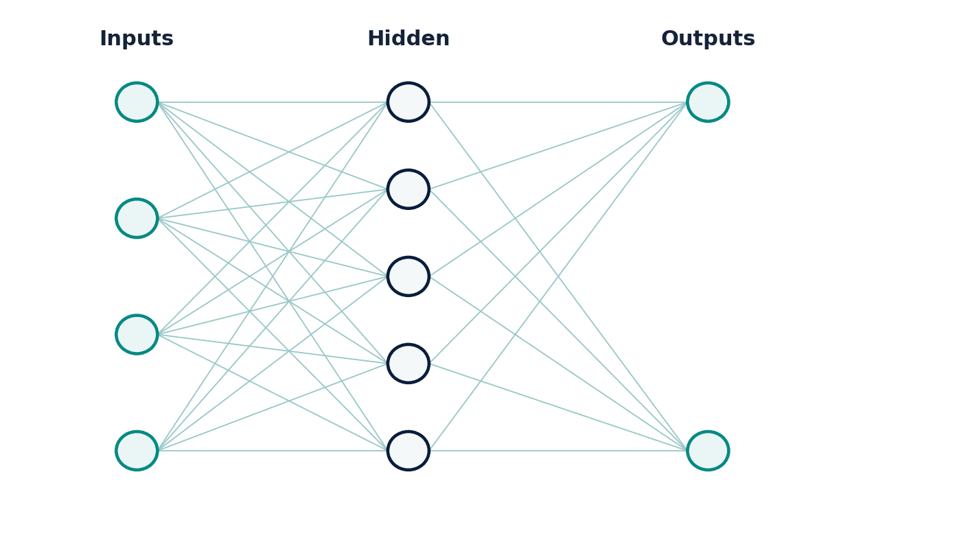
A neuron forms a weighted sum of inputs, adds a bias, and applies an activation function. A layer transforms a vector into another representation; multiple layers compose these transformations into a flexible nonlinear function. Without nonlinear activations, stacked linear layers collapse into one linear mapping. ReLU is common because it is simple and supports gradient-based optimization, while output activations depend on the task.
Key terms
- neurons, activations, layers, and forward passes
- A core idea in Chapter 49 that students apply carefully in economic analysis.
- backpropagation and optimization
- A core idea in Chapter 49 that students apply carefully in economic analysis.
- Train a small PyTorch network
- A core idea in Chapter 49 that students apply carefully in economic analysis.
- learning curves, regularization, and validation
- A core idea in Chapter 49 that students apply carefully in economic analysis.
- Prerequisites: Chapters 8, 14, and 28
- A core idea in Chapter 49 that students apply carefully in economic analysis.
- Key terms: neuron, activation, forward pass, backpropagation, epoch, regularization
- A core idea in Chapter 49 that students apply carefully in economic analysis.
Analytical workflow
Interpret the expression in words and units before using it in a claim.
Example
Interpretation. The network learns a nonlinear approximation on a small CPU-friendly problem. The exact final loss may vary slightly by software and hardware.
Prerequisites
- Complete the preceding course chapters or review their summaries as needed.
Full theory and examples
49.2
A neural network composes transformations
A neuron forms a weighted sum of inputs, adds a bias, and applies an activation function. A layer transforms a vector into another representation; multiple layers compose these transformations into a flexible nonlinear function. Without nonlinear activations, stacked linear layers collapse into one linear mapping. ReLU is common because it is simple and supports gradient-based optimization, while output activations depend on the task.
49.3
Backpropagation is organized chain-rule accounting
A forward pass computes predictions and loss. Backpropagation applies the chain rule from the loss back through each operation to calculate parameter gradients. An optimizer updates weights. Batches approximate the full-data gradient, and epochs count passes through the training data. Modern frameworks automate derivatives, but shape, scale, target coding, and loss selection remain human responsibilities (PyTorch Contributors 2026; Goodfellow, Bengio, and Courville 2016).
49.4
Learning curves reveal optimization and generalization
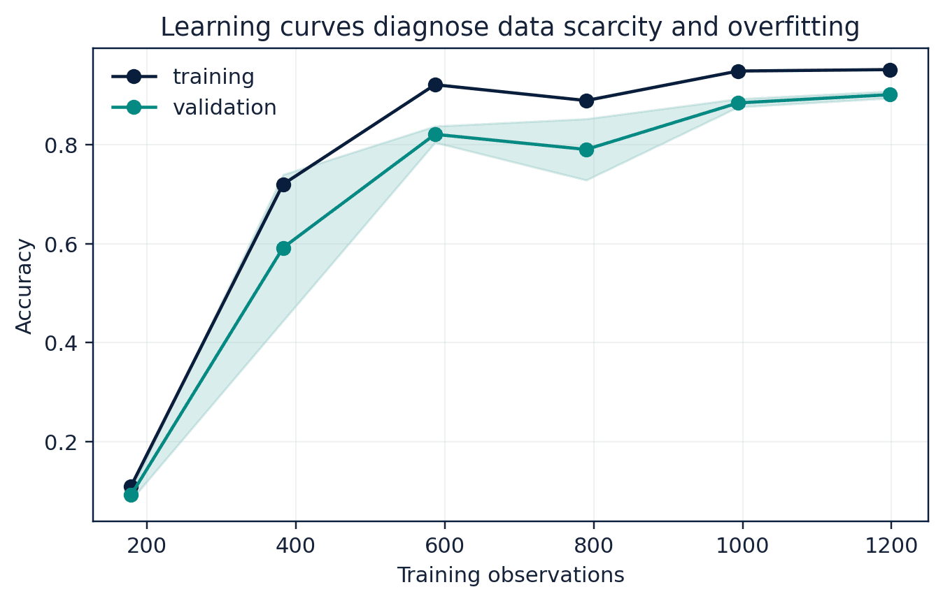
Training loss should generally fall, but validation loss determines whether performance transfers. A widening gap can indicate overfitting. Dropout, weight decay, early stopping, data augmentation, and simpler architectures can help. Deep models are not automatically superior on small tabular economic data, where linear or tree-based models often provide stronger baselines and clearer diagnostics.
49.5
Core equations
Neuron
The activation phi transforms a weighted input plus bias.
Cross-entropy
Classification loss penalizes low predicted probability for the observed class.
49.6
Python demonstrations
49.6.1
Demonstration 30.1: A small PyTorch network
Verified output
Interpretation. The network learns a nonlinear approximation on a small CPU-friendly problem. The exact final loss may vary slightly by software and hardware.
49.6.2
Demonstration 30.2: Separate training from evaluation
Verified output
Interpretation. Evaluation mode and no_grad disable training-specific behaviour and gradient storage during prediction.
49.7
Visual evidence
49.8
Reference table
Why This Matters
Neural networks are flexible function approximators whose usefulness depends on data, validation, computation, and governance.
Common Mistake
Choosing a large network before establishing a linear or tree-based baseline.
Ceteris LAB Tip
Log training and validation metrics every epoch, but select the checkpoint using validation performance rather than training loss.
R-to-Python / Source Bridge
The chapter adapts IntroAI session 7, including neurons, activations, cross-entropy, backpropagation, and PyTorch, while keeping required examples small enough for CPU execution (Sharifi-Zarchi and contributors 2026).
| Component | Purpose | Typical choice |
|---|---|---|
| hidden activation | nonlinearity | ReLU |
| output activation | match target support | identity, sigmoid, softmax |
| loss | training objective | MSE or cross-entropy |
| optimizer | parameter update | SGD or Adam |
| regularization | reduce overfitting | weight decay/dropout |
| validation | generalization signal | held-out loss/metric |
Visual evidence
Additional Python demonstrations
Live Python
Source demonstration 2
Source demonstration 2
Stdout
Run Python to see results here.
Status / stderr
Ready to run Python in your browser.
Line-by-line guide
- Line 1Load a Python library needed for data work or regression.
- Line 3Create or update a Python object used in the analysis.
- Line 4Create or update a Python object used in the analysis.
- Line 5Create or update a Python object used in the analysis.
- Line 6Display a result so students can inspect the output.
- Line 7Display a result so students can inspect the output.
Verified source output
0.01343
[-1.024999976158142, 0.0, 1.0119999647140503]
Interpretation. The network learns a nonlinear approximation on a small CPU-friendly problem. The exact final loss may vary slightly by software and hardware.
Interpretation. Evaluation mode and no_grad disable training-specific behaviour and gradient storage during prediction.
Guided practice
- 1Re-run Demonstration 30.1 and change one input while keeping the analytical question fixed.
- 2Explain in two sentences how the output supports, or fails to support, the chapter opening question.
- 3Add one validation check that would prevent a plausible error.
Exercises
- 1Build a one-hidden-layer regression network.
- 2Compare ReLU and tanh activations.
- 3Plot training and validation loss.
- 4Add weight decay and discuss the change.
Source and downloads
Chapter 49 of Fundamentals of Python for Financial Econometrics by Mohammad Safavi, Ph.D.. The lesson is an original Ceteris Lab web adaptation of the supplied publication package.
Live Python
Neural Networks and Deep Learning for Economic Data: live Python
Neural Networks and Deep Learning for Economic Data: live Python
Stdout
Run Python to see results here.
Status / stderr
Ready to run Python in your browser.
Line-by-line guide
- Line 1Load a Python library needed for data work or regression.
- Line 3Create or update a Python object used in the analysis.
- Line 4Create or update a Python object used in the analysis.
- Line 5Create or update a Python object used in the analysis.
- Line 6Create or update a Python object used in the analysis.
- Line 7Create or update a Python object used in the analysis.
- Line 8Create or update a Python object used in the analysis.
- Line 9Create or update a Python object used in the analysis.
- Line 10Create or update a Python object used in the analysis.
- Line 11Create or update a Python object used in the analysis.
- Line 12Display a result so students can inspect the output.
- Line 14Create or update a Python object used in the analysis.
- Line 15Create or update a Python object used in the analysis.
- Line 16Create or update a Python object used in the analysis.
- Line 17Display a result so students can inspect the output.
- Line 18Display a result so students can inspect the output.
Python walkthrough
- 1`import numpy as np`: Loads a package or function used by the analysis.
- 2`rng = np.random.default_rng(49)`: Creates or updates a named object used by later steps.
- 3`X = np.linspace(-1, 1, 200).reshape(-1, 1)`: Creates or updates a named object used by later steps.
- 4`y = 2 * X[:, 0] + 0.3 * np.sin(6 * X[:, 0])`: Creates or updates a named object used by later steps.
- 5`hidden_weights = rng.normal(size=(1, 12))`: Creates or updates a named object used by later steps.
- 6`hidden_bias = rng.normal(scale=0.25, size=12)`: Creates or updates a named object used by later steps.
- 7`hidden = np.tanh(X @ hidden_weights + hidden_bias)`: Creates or updates a named object used by later steps.
- 8`design = np.column_stack([np.ones(len(X)), hidden])`: Creates or updates a named object used by later steps.
- 9`output_weights = np.linalg.lstsq(design, y, rcond=None)[0]`: Creates or updates a named object used by later steps.
- 10`fitted = design @ output_weights`: Creates or updates a named object used by later steps.
- 11`print("Training RMSE:", round(float(np.sqrt(np.mean((y - fitted) ** 2))), 4))`: Displays a result so it can be checked and interpreted.
- 12`new_x = np.array([[-0.5], [0.0], [0.5]])`: Creates or updates a named object used by later steps.
Live notebook
Run this lesson as a notebook
Open an editable notebook cell-by-cell, run Python in the browser, and download the `.ipynb` file for later.
Related dataset
Ceteris Lab teaching sample
Estimated time
25 to 40 min
Packages
pandas, numpy
Expected output
Printed Python results that can be compared with the lesson explanation.
Learning goals
- Load and inspect Ceteris Lab teaching sample.
- Run the Python cells connected to Neural Networks and Deep Learning for Economic Data.
- Interpret the output using neurons, activations, layers, and forward passes and backpropagation and optimization.
Common errors
- File not found: check that wage_sample.csv is installed or use the course data folder.
- Package import error: use the browser notebook first, then download for local Jupyter if your local packages differ.
- Column name error: compare your variable names with the dataset variables listed for this notebook.
Dataset path helper
import pandas as pd

df = pd.read_csv("/data/wage_sample.csv")
df.head()
Interactive activity
Chapter 49 interactive
Model governance check
What is the safest basis for evaluating an ML or AI result?
Immediate feedback
Choose a decision, then test how the claim changes as evidence becomes stronger or weaker.
Try it yourself
Write one plain-English sentence explaining the main idea from this lesson.
Common mistakes
Check these before you move on.
Return to the lesson assumptions, units, diagnostics, and source evidence to replace this shortcut with a defensible interpretation.
Quick quiz
Which statement best answers the Chapter 49 opening question: How does a stack of simple differentiable units learn a nonlinear mapping, and how do we know it has not merely memorized the training sample?
Quick quiz
Which practice should be avoided when applying Neural Networks and Deep Learning for Economic Data?
Quick quiz
What is the most defensible way to interpret the Python demonstration?
Quick quiz
Why does Chapter 49 matter in an applied econometrics workflow?
Key takeaway
Neural networks compose linear transformations and nonlinear activations. Backpropagation computes gradients through the computation graph. Validation and regularization are essential for generalization.