Lesson 41
Asymmetric, Advanced, and Realized Volatility
Big question
Why can equally large negative and positive shocks have different volatility consequences, and what can intraday or OHLC data add?
Lesson progress
Complete checkpoints as you learn
Learning objectives
- Compare EGARCH, GJR-GARCH, APARCH, and GARCH-M concepts.
- Interpret leverage and news-impact curves.
- Calculate rolling, EWMA, realized, and range-based volatility.
- Discuss microstructure noise and overnight information.
- Prerequisites: Chapter 21.
- Key terms: EGARCH, GJR-GARCH, APARCH, leverage effect, realized volatility, OHLC estimator.
Simple explanation
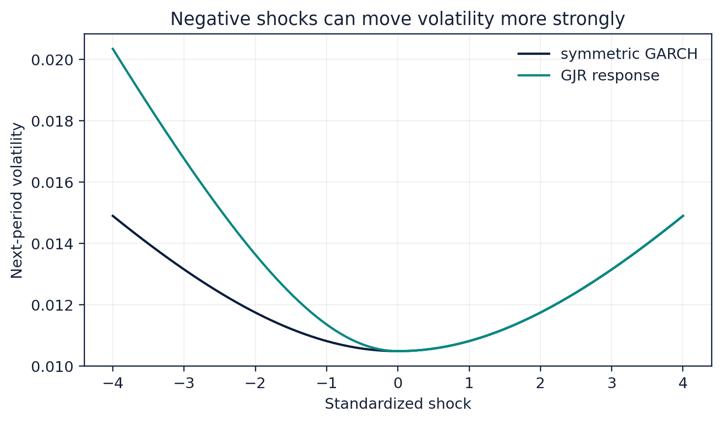
Negative equity shocks often increase subsequent volatility more than positive shocks of the same magnitude. EGARCH models log variance and permits asymmetric standardized-shock effects without imposing positivity constraints directly (Nelson 1991). GJR-GARCH adds an indicator for negative innovations. APARCH generalizes the power applied to volatility and shock magnitude. Parameter names and signs differ across software, so interpretation should follow the exact implemented equation.
Key terms
- Compare EGARCH, GJR-GARCH, APARCH, and GARCH-M concepts
- A core idea in Chapter 41 that students apply carefully in economic analysis.
- leverage and news-impact curves
- A core idea in Chapter 41 that students apply carefully in economic analysis.
- Calculate rolling, EWMA, realized, and range-based volatility
- A core idea in Chapter 41 that students apply carefully in economic analysis.
- Discuss microstructure noise and overnight information
- A core idea in Chapter 41 that students apply carefully in economic analysis.
- Prerequisites: Chapter 21
- A core idea in Chapter 41 that students apply carefully in economic analysis.
- Key terms: EGARCH, GJR-GARCH, APARCH, leverage effect, realized volatility, OHLC estimator
- A core idea in Chapter 41 that students apply carefully in economic analysis.
Analytical workflow
Interpret the expression in words and units before using it in a claim.
Example
Interpretation. Recent squared returns receive greater weight, while the recursion never fully forgets earlier variance.
Prerequisites
- Complete the preceding course chapters or review their summaries as needed.
Full theory and examples
41.2
Asymmetry belongs in the variance equation
Negative equity shocks often increase subsequent volatility more than positive shocks of the same magnitude. EGARCH models log variance and permits asymmetric standardized-shock effects without imposing positivity constraints directly (Nelson 1991). GJR-GARCH adds an indicator for negative innovations. APARCH generalizes the power applied to volatility and shock magnitude. Parameter names and signs differ across software, so interpretation should follow the exact implemented equation.
41.3
Realized measures use more of the day
Realized variance sums squared intraday returns. Under ideal continuous sampling it approximates quadratic variation, but extremely high frequency introduces bid-ask bounce and other microstructure noise. Overnight price changes carry information that an intraday sum can miss. Sampling intervals, market hours, and data cleaning therefore become part of the volatility estimator.
41.4
OHLC estimators trade assumptions for efficiency
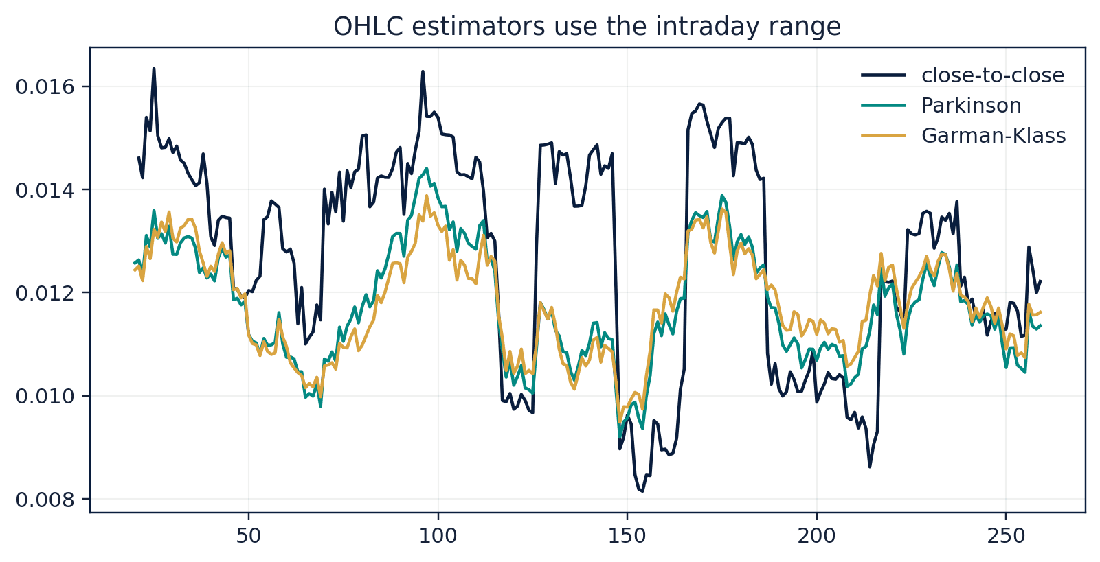
High, low, open, and close prices contain more intraday information than close-to-close returns. Parkinson, Garman-Klass, Rogers-Satchell, and Yang-Zhang estimators use different combinations and assumptions about drift and overnight gaps (Garman and Klass 1980; Yang and Zhang 2000). Corporate actions must be handled consistently. Comparing several measures is usually more informative than declaring one universally best.
41.5
Core equations
Realized variance
Intraday squared returns are summed within a day.
Parkinson variance
The high-low range provides an efficient estimator under a driftless diffusion idealization.
41.6
Python demonstrations
41.6.1
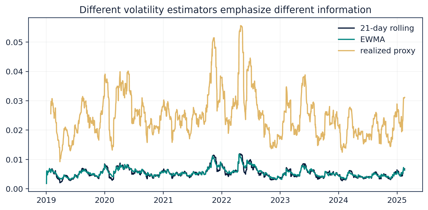
Demonstration 22.1: EWMA variance recursion
Verified output
Interpretation. Recent squared returns receive greater weight, while the recursion never fully forgets earlier variance.
41.6.2
Demonstration 22.2: Parkinson and Garman-Klass estimates
Verified output
Interpretation. The estimators use the same OHLC day but weight its range and open-to-close movement differently.
41.7
Visual evidence
41.8
Reference table
Why This Matters
Alternative volatility measures reveal how much the result depends on data frequency, asymmetry, and model assumptions.
Common Mistake
Calling every negative-return coefficient a “leverage effect” without checking the package equation and indicator definition.
Ceteris LAB Tip
Draw a news-impact curve from the fitted equation. The picture often clarifies asymmetry better than a coefficient table.
R-to-Python / Source Bridge
The source “More Volatility Models” and “Alternative Approaches” lectures cover GARCH-M, EGARCH, GJR/TGARCH, APARCH, realized volatility, and OHLC estimators. This chapter consolidates them into one tested Python workflow (Tsay 2013).
| Method | Information used | Main limitation |
|---|---|---|
| rolling SD | recent close returns | window choice |
| EWMA | all past returns with decay | fixed decay parameter |
| GARCH | model-based shocks and variance | specification risk |
| realized variance | intraday returns | microstructure noise and overnight gap |
| Yang-Zhang | open/high/low/close | corporate actions and assumptions |
Visual evidence
Additional Python demonstrations
Live Python
Source demonstration 2
Source demonstration 2
Stdout
Run Python to see results here.
Status / stderr
Ready to run Python in your browser.
Line-by-line guide
- Line 1Load a Python library needed for data work or regression.
- Line 3Create or update a Python object used in the analysis.
- Line 4Create a log version of the variable so coefficients can be read approximately as percentages.
- Line 5Create a log version of the variable so coefficients can be read approximately as percentages.
- Line 6Create a log version of the variable so coefficients can be read approximately as percentages.
- Line 7Create a log version of the variable so coefficients can be read approximately as percentages.
- Line 8Display a result so students can inspect the output.
Verified source output
[0.0133 0.0138 0.0134 0.0135]
0.001717 0.002042
Interpretation. Recent squared returns receive greater weight, while the recursion never fully forgets earlier variance.
Interpretation. The estimators use the same OHLC day but weight its range and open-to-close movement differently.
Guided practice
- 1Re-run Demonstration 22.1 and change one input while keeping the analytical question fixed.
- 2Explain in two sentences how the output supports, or fails to support, the chapter opening question.
- 3Add one validation check that would prevent a plausible error.
Exercises
- 1Calculate a rolling and EWMA volatility series.
- 2Compare Gaussian GARCH and GJR-GARCH.
- 3Compute realized variance at two sampling intervals.
- 4Implement Parkinson and Yang-Zhang estimators on adjusted OHLC data.
Source and downloads
Chapter 41 of Fundamentals of Python for Financial Econometrics by Mohammad Safavi, Ph.D.. The lesson is an original Ceteris Lab web adaptation of the supplied publication package.
Live Python
Asymmetric, Advanced, and Realized Volatility: live Python
Asymmetric, Advanced, and Realized Volatility: live Python
Stdout
Run Python to see results here.
Status / stderr
Ready to run Python in your browser.
Line-by-line guide
- Line 1Load a Python library needed for data work or regression.
- Line 3Create or update a Python object used in the analysis.
- Line 4Create or update a Python object used in the analysis.
- Line 5Create or update a Python object used in the analysis.
- Line 6Create or update a Python object used in the analysis.
- Line 7Run this Python instruction as part of the lesson workflow.
- Line 8Create or update a Python object used in the analysis.
- Line 9Run this Python instruction as part of the lesson workflow.
- Line 10Display a result so students can inspect the output.
Python walkthrough
- 1`import numpy as np`: Loads a package or function used by the analysis.
- 2`returns = np.array([0.01, -0.02, 0.005, 0.015])`: Creates or updates a named object used by later steps.
- 3`lam = 0.94`: Creates or updates a named object used by later steps.
- 4`variance = returns.var()`: Creates or updates a named object used by later steps.
- 5`path = []`: Creates or updates a named object used by later steps.
- 6`for r in returns:`: Repeats the indented calculation across observations or simulation draws.
- 7`variance = lam * variance + (1-lam) * r**2`: Creates or updates a named object used by later steps.
- 8`path.append(variance)`: Executes the next transparent step in the workflow.
- 9`print(np.round(np.sqrt(path), 4))`: Displays a result so it can be checked and interpreted.
Live notebook
Run this lesson as a notebook
Open an editable notebook cell-by-cell, run Python in the browser, and download the `.ipynb` file for later.
Related dataset
Ceteris Lab teaching sample
Estimated time
25 to 40 min
Packages
pandas, numpy
Expected output
Printed Python results that can be compared with the lesson explanation.
Learning goals
- Load and inspect Ceteris Lab teaching sample.
- Run the Python cells connected to Asymmetric, Advanced, and Realized Volatility.
- Interpret the output using Compare EGARCH, GJR-GARCH, APARCH, and GARCH-M concepts and leverage and news-impact curves.
Common errors
- File not found: check that wage_sample.csv is installed or use the course data folder.
- Package import error: use the browser notebook first, then download for local Jupyter if your local packages differ.
- Column name error: compare your variable names with the dataset variables listed for this notebook.
Dataset path helper
import pandas as pd

df = pd.read_csv("/data/wage_sample.csv")
df.head()
Interactive activity
Chapter 41 interactive
Assumption stress test
What should determine the strength of an econometric claim?
Immediate feedback
Choose a decision, then test how the claim changes as evidence becomes stronger or weaker.
Try it yourself
Write one plain-English sentence explaining the main idea from this lesson.
Common mistakes
Check these before you move on.
Return to the lesson assumptions, units, diagnostics, and source evidence to replace this shortcut with a defensible interpretation.
Quick quiz
Which statement best answers the Chapter 41 opening question: Why can equally large negative and positive shocks have different volatility consequences, and what can intraday or OHLC data add?
Quick quiz
Which practice should be avoided when applying Asymmetric, Advanced, and Realized Volatility?
Quick quiz
What is the most defensible way to interpret the Python demonstration?
Quick quiz
Why does Chapter 41 matter in an applied econometrics workflow?
Key takeaway
Asymmetric models allow shock sign to affect future variance. Realized volatility uses intraday information but faces microstructure noise. Range-based estimators improve information use under specific assumptions.