Lesson 14
Probability, Simulation, and Statistical Inference
Big question
How can uncertainty be represented, simulated, and summarized without pretending that one sample is the population?
Lesson progress
Complete checkpoints as you learn
Learning objectives
- Work with random variables and common distributions.
- Use Monte Carlo simulation.
- Explain sampling distributions and standard errors.
- Interpret confidence intervals, tests, and power.
- Prerequisites: Chapter 13 and basic algebra.
- Key terms: random variable, distribution, Monte Carlo, standard error, confidence interval, p-value.
Simple explanation
A probability distribution assigns relative plausibility to possible outcomes under stated assumptions. The normal distribution is useful for averages and measurement errors; the binomial for counts of successes; the Student-t for heavier-tailed standardized quantities; and the lognormal for positive multiplicative processes. Real data need not follow any textbook distribution exactly. A distribution is a working model whose implications should be checked.
Key terms
- Work with random variables and common distributions
- A core idea in Chapter 14 that students apply carefully in economic analysis.
- Monte Carlo simulation
- A core idea in Chapter 14 that students apply carefully in economic analysis.
- sampling distributions and standard errors
- A core idea in Chapter 14 that students apply carefully in economic analysis.
- confidence intervals, tests, and power
- A core idea in Chapter 14 that students apply carefully in economic analysis.
- Prerequisites: Chapter 13 and basic algebra
- A core idea in Chapter 14 that students apply carefully in economic analysis.
- Key terms: random variable, distribution, Monte Carlo, standard error, confidence interval, p-value
- A core idea in Chapter 14 that students apply carefully in economic analysis.
Analytical workflow
Interpret the expression in words and units before using it in a claim.
Example
Interpretation. The estimate is close to the theoretical upper-tail probability of 0.025, with small Monte Carlo error.
Prerequisites
- Complete the preceding course chapters or review their summaries as needed.
Full theory and examples
14.2
Probability describes a model of uncertainty
A probability distribution assigns relative plausibility to possible outcomes under stated assumptions. The normal distribution is useful for averages and measurement errors; the binomial for counts of successes; the Student-t for heavier-tailed standardized quantities; and the lognormal for positive multiplicative processes. Real data need not follow any textbook distribution exactly. A distribution is a working model whose implications should be checked.
14.3
Simulation turns assumptions into observable consequences
Monte Carlo simulation draws repeated outcomes from a model and approximates quantities that may be difficult to calculate analytically. The method supports option pricing, forecast intervals, power analysis, and risk measurement. More replications reduce simulation noise at a square-root rate, so ten times more computation does not produce ten times more precision. Seeds make examples repeatable; multiple seeds test whether a conclusion is fragile.
14.4
Inference concerns repeated-sample behaviour
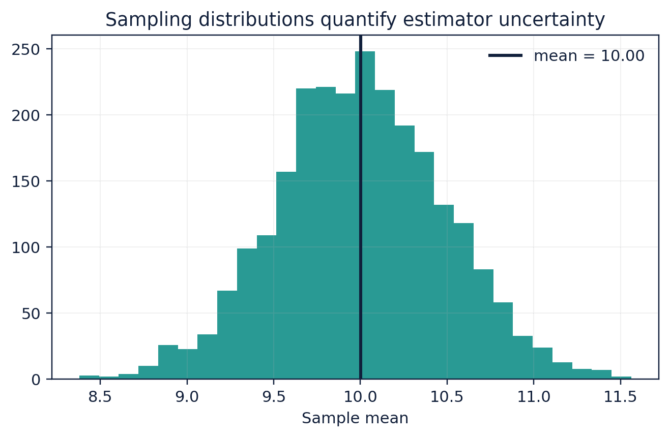
A standard error estimates how a statistic would vary across hypothetical repeated samples. A confidence interval is constructed by a procedure with a long-run coverage property; it is not automatically a probability statement about a fixed parameter. A p-value measures compatibility between data and a null model, not the probability that the null is true. Statistical significance should be paired with effect size, uncertainty, design, and practical relevance.
14.5
Core equations
Standard error of the mean
Under standard independent-sampling conditions, precision improves with the square root of sample size.
14.6
Python demonstrations
14.6.1
Demonstration 14.1: Monte Carlo estimate of a probability
Verified output
Interpretation. The estimate is close to the theoretical upper-tail probability of 0.025, with small Monte Carlo error.
14.6.2
Demonstration 14.2: A confidence interval for a mean
Verified output
Interpretation. The interval is wider than a normal-based interval because the small sample uses a Student-t critical value.
14.7
Visual evidence
14.8
Reference table
Why This Matters
Inference organizes uncertainty around estimates, forecasts, and decisions.
Common Mistake
Interpreting a p-value of 0.03 as a 3 percent probability that the null hypothesis is true.
Ceteris LAB Tip
Report effect size and interval before discussing a significance threshold.
R-to-Python / Source Bridge
The book adds probability and inference prerequisites that the advanced source notes often assumed, allowing beginners to enter later econometric chapters safely.
| Quantity | What varies? | Interpretation |
|---|---|---|
| standard deviation | individual observations | spread in data or model |
| standard error | statistic across samples | estimation precision |
| confidence interval | procedure across samples | coverage under assumptions |
| p-value | test statistic under null | compatibility with null model |
| power | test decision under alternative | probability of detecting specified effect |
Visual evidence
Additional Python demonstrations
Live Python
Source demonstration 2
Source demonstration 2
Stdout
Run Python to see results here.
Status / stderr
Ready to run Python in your browser.
Line-by-line guide
- Line 1Load a Python library needed for data work or regression.
- Line 2Load a Python library needed for data work or regression.
- Line 4Create or update a Python object used in the analysis.
- Line 5Create or update a Python object used in the analysis.
- Line 6Create or update a Python object used in the analysis.
- Line 7Create or update a Python object used in the analysis.
- Line 8Display a result so students can inspect the output.
Verified source output
0.0249
2.333 (np.float64(2.062), np.float64(2.604))
Interpretation. The estimate is close to the theoretical upper-tail probability of 0.025, with small Monte Carlo error.
Interpretation. The interval is wider than a normal-based interval because the small sample uses a Student-t critical value.
Guided practice
- 1Re-run Demonstration 14.1 and change one input while keeping the analytical question fixed.
- 2Explain in two sentences how the output supports, or fails to support, the chapter opening question.
- 3Add one validation check that would prevent a plausible error.
Exercises
- 1Simulate a binomial proportion.
- 2Show how Monte Carlo error changes with replications.
- 3Compute a t confidence interval.
- 4Explain statistical versus practical significance in one example.
Source and downloads
Chapter 14 of Fundamentals of Python for Financial Econometrics by Mohammad Safavi, Ph.D.. The lesson is an original Ceteris Lab web adaptation of the supplied publication package.
Live Python
Probability, Simulation, and Statistical Inference: live Python
Probability, Simulation, and Statistical Inference: live Python
Stdout
Run Python to see results here.
Status / stderr
Ready to run Python in your browser.
Line-by-line guide
- Line 1Load a Python library needed for data work or regression.
- Line 3Create or update a Python object used in the analysis.
- Line 4Create or update a Python object used in the analysis.
- Line 5Create or update a Python object used in the analysis.
- Line 6Display a result so students can inspect the output.
Python walkthrough
- 1`import numpy as np`: Loads a package or function used by the analysis.
- 2`rng = np.random.default_rng(1401)`: Creates or updates a named object used by later steps.
- 3`draws = rng.normal(0, 1, 100_000)`: Creates or updates a named object used by later steps.
- 4`probability = np.mean(draws > 1.96)`: Creates or updates a named object used by later steps.
- 5`print(round(probability, 4))`: Displays a result so it can be checked and interpreted.
Live notebook
Run this lesson as a notebook
Open an editable notebook cell-by-cell, run Python in the browser, and download the `.ipynb` file for later.
Related dataset
Ceteris Lab teaching sample
Estimated time
35 to 55 min
Packages
pandas, numpy, statsmodels, patsy, scipy
Expected output
A regression or inference table with coefficients, uncertainty, and short interpretation notes.
Learning goals
- Load and inspect Ceteris Lab teaching sample.
- Run the Python cells connected to Probability, Simulation, and Statistical Inference.
- Interpret the output using Work with random variables and common distributions and Monte Carlo simulation.
Common errors
- File not found: check that wage_sample.csv is installed or use the course data folder.
- Package import error: use the browser notebook first, then download for local Jupyter if your local packages differ.
- Column name error: compare your variable names with the dataset variables listed for this notebook.
Dataset path helper
import pandas as pd

df = pd.read_csv("/data/wage_sample.csv")
df.head()
Interactive activity
Chapter 14 interactive
Data evidence planner
Which choice makes an exploratory result easier to defend?
Immediate feedback
Choose a decision, then test how the claim changes as evidence becomes stronger or weaker.
Try it yourself
Write one plain-English sentence explaining the main idea from this lesson.
Common mistakes
Check these before you move on.
Return to the lesson assumptions, units, diagnostics, and source evidence to replace this shortcut with a defensible interpretation.
Quick quiz
Which statement best answers the Chapter 14 opening question: How can uncertainty be represented, simulated, and summarized without pretending that one sample is the population?
Quick quiz
Which practice should be avoided when applying Probability, Simulation, and Statistical Inference?
Quick quiz
What is the most defensible way to interpret the Python demonstration?
Quick quiz
Why does Chapter 14 matter in an applied econometrics workflow?
Key takeaway
Probability models uncertainty under assumptions. Simulation approximates model implications. Inference requires careful interpretation of standard errors, intervals, and tests.