Lesson 43
Stochastic Processes and Option Pricing
Big question
How can continuous-time uncertainty be simulated and translated into a no-arbitrage option value?
Lesson progress
Complete checkpoints as you learn
Learning objectives
- Simulate Brownian motion and geometric Brownian motion.
- Explain Ito’s lemma intuitively.
- Calculate European option payoffs and Black-Scholes prices.
- Use Monte Carlo and sensitivity analysis.
- Prerequisites: Probability, logarithms, derivatives, and Chapter 22.
- Key terms: Brownian motion, diffusion, Ito’s lemma, geometric Brownian motion, Black-Scholes, Greek.
Simple explanation
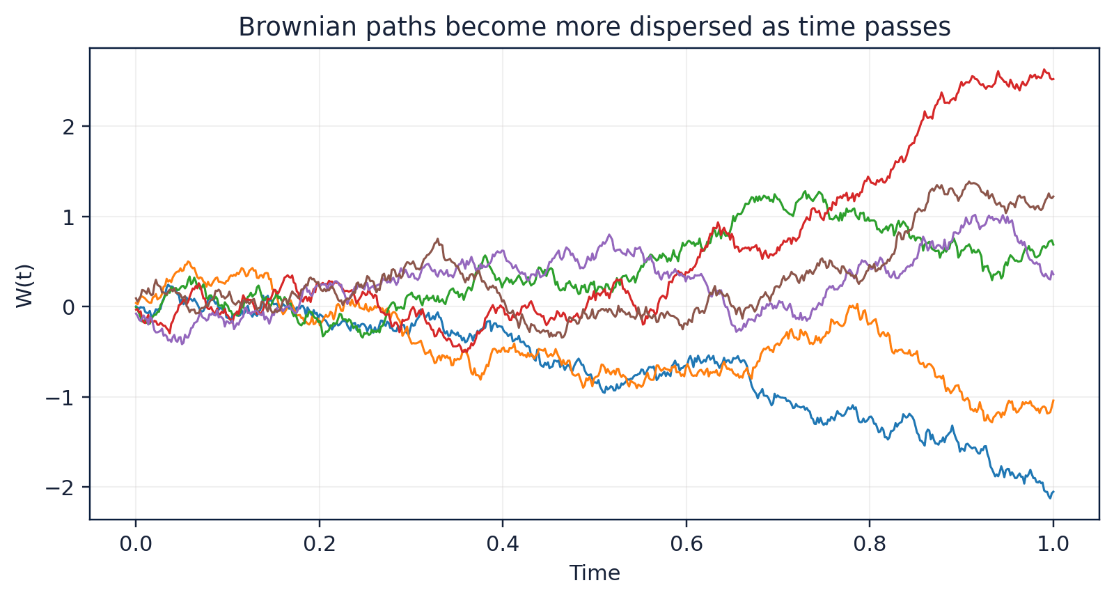
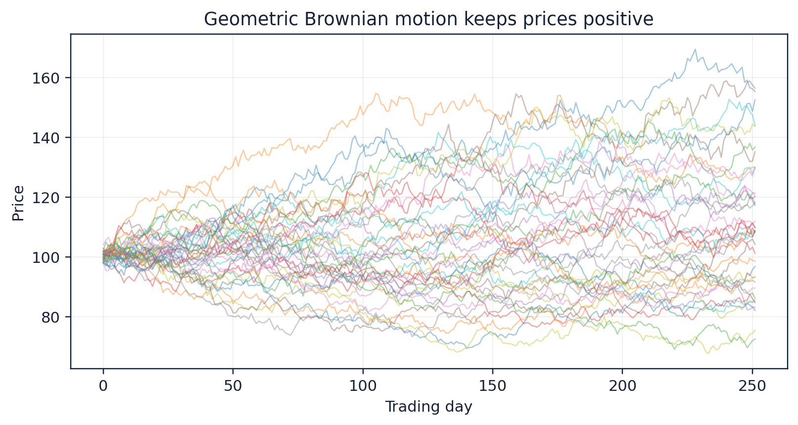
A standard Brownian motion begins at zero, has independent normally distributed increments, and variance that grows with elapsed time. Its paths are continuous but nowhere classically differentiable. A generalized diffusion adds drift and a volatility scale. Geometric Brownian motion multiplies both by the current price, keeping simulated prices positive under the exact lognormal solution.
Key terms
- Simulate Brownian motion and geometric Brownian motion
- A core idea in Chapter 43 that students apply carefully in economic analysis.
- Ito’s lemma intuitively
- A core idea in Chapter 43 that students apply carefully in economic analysis.
- Calculate European option payoffs and Black-Scholes prices
- A core idea in Chapter 43 that students apply carefully in economic analysis.
- Monte Carlo and sensitivity analysis
- A core idea in Chapter 43 that students apply carefully in economic analysis.
- Prerequisites: Probability, logarithms, derivatives, and Chapter 22
- A core idea in Chapter 43 that students apply carefully in economic analysis.
- Key terms: Brownian motion, diffusion, Ito’s lemma, geometric Brownian motion, Black-Scholes, Greek
- A core idea in Chapter 43 that students apply carefully in economic analysis.
Chapter 43 model
Interpret the expression in words and units before using it in a claim.
Example
Interpretation. One path is a possible model realization, not a forecast. Many paths are needed for a distribution or Monte Carlo estimate.
Prerequisites
- Complete the preceding course chapters or review their summaries as needed.
Full theory and examples
43.2
Brownian motion accumulates random increments
A standard Brownian motion begins at zero, has independent normally distributed increments, and variance that grows with elapsed time. Its paths are continuous but nowhere classically differentiable. A generalized diffusion adds drift and a volatility scale. Geometric Brownian motion multiplies both by the current price, keeping simulated prices positive under the exact lognormal solution.
43.3
Ito’s lemma adds a variance correction
Ordinary calculus ignores squared infinitesimal changes, but a Brownian increment has magnitude proportional to the square root of time, so its square contributes at order dt. Ito’s lemma therefore adds a second-derivative term. Applied to log price under geometric Brownian motion, it produces drift mu minus one-half sigma squared. The result explains why expected arithmetic return and expected log growth differ.
43.4
Black-Scholes is a model, not a market law
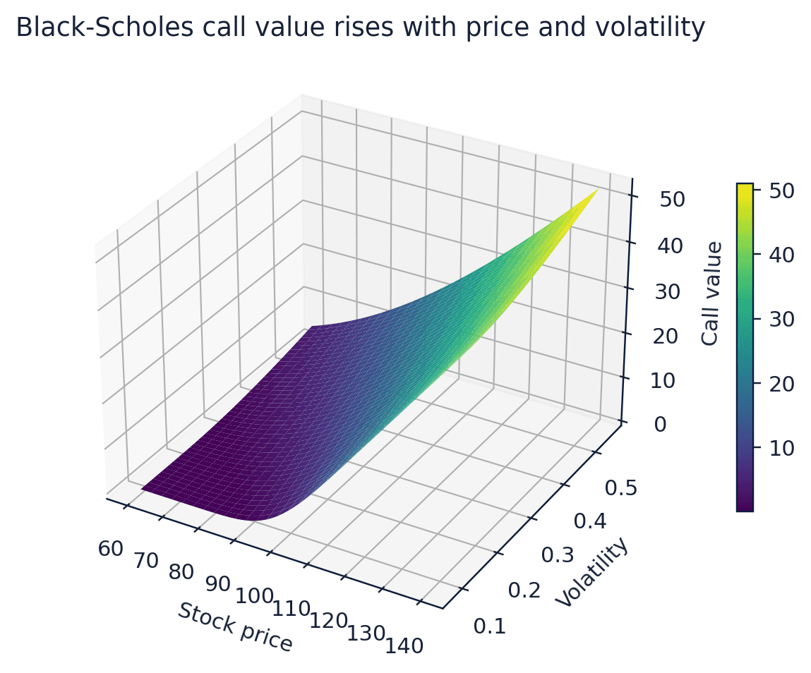
The Black-Scholes-Merton framework derives a European option price by constructing a locally hedged portfolio under assumptions including continuous trading, frictionless markets, constant volatility and rate, and a diffusion price process (Black and Scholes 1973; Merton 1973). Real markets violate these assumptions. The formula remains a useful benchmark, and sensitivity measures such as delta and vega reveal how the benchmark changes when inputs move.
43.5
Core equations
Geometric Brownian motion
The exact log-price increment is normal with drift (mu-sigma^2/2)dt and variance sigma^2 dt.
European call
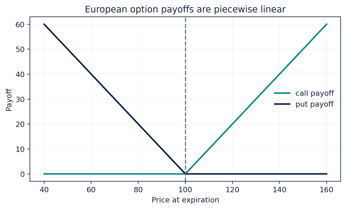
The Black-Scholes call price under the standard no-dividend assumptions.
43.6
Python demonstrations
43.6.1
Demonstration 24.1: Simulate geometric Brownian motion
Verified output
Interpretation. One path is a possible model realization, not a forecast. Many paths are needed for a distribution or Monte Carlo estimate.
43.6.2
Demonstration 24.2: Black-Scholes call price
Verified output
Interpretation. The value is conditional on the model inputs and assumptions. It is not a trading recommendation or a guarantee of market price.
43.7
Visual evidence
43.8
Reference table
Why This Matters
Stochastic-process models connect return dynamics, derivative valuation, simulation, and risk management.
Common Mistake
Using an annual volatility with time measured in days, or a daily volatility with time measured in years.
Ceteris LAB Tip
Write all time and rate units beside the formula before calculating an option value.
R-to-Python / Source Bridge
The source option-pricing lecture develops Brownian motion, Ito’s lemma, geometric Brownian motion, hedging, and Black-Scholes. Every R simulation is replaced by reproducible NumPy code and original sensitivity graphics (Tsay 2013).
| Input | Effect on call price | Caution |
|---|---|---|
| spot S | usually positive | moneyness matters |
| strike K | usually negative | contract definition |
| time T | often positive | theta can vary |
| rate r | usually positive for calls | yield conventions |
| volatility sigma | positive vega | implied volatility varies by strike and maturity |
Visual evidence
Additional Python demonstrations
Live Python
Source demonstration 2
Source demonstration 2
Stdout
Run Python to see results here.
Status / stderr
Ready to run Python in your browser.
Line-by-line guide
- Line 1Load a Python library needed for data work or regression.
- Line 3Run this Python instruction as part of the lesson workflow.
- Line 4Run this Python instruction as part of the lesson workflow.
- Line 6Run this Python instruction as part of the lesson workflow.
- Line 7Create or update a Python object used in the analysis.
- Line 8Create or update a Python object used in the analysis.
- Line 9Run this Python instruction as part of the lesson workflow.
- Line 11Create or update a Python object used in the analysis.
- Line 12Display a result so students can inspect the output.
Verified source output
59.88
9.4134
Interpretation. One path is a possible model realization, not a forecast. Many paths are needed for a distribution or Monte Carlo estimate.
Interpretation. The value is conditional on the model inputs and assumptions. It is not a trading recommendation or a guarantee of market price.
Guided practice
- 1Re-run Demonstration 24.1 and change one input while keeping the analytical question fixed.
- 2Explain in two sentences how the output supports, or fails to support, the chapter opening question.
- 3Add one validation check that would prevent a plausible error.
Exercises
- 1Simulate four Brownian paths.
- 2Verify that Brownian variance increases with time.
- 3Compare Monte Carlo and Black-Scholes call values.
- 4Plot call value against volatility and time.
Source and downloads
Chapter 43 of Fundamentals of Python for Financial Econometrics by Mohammad Safavi, Ph.D.. The lesson is an original Ceteris Lab web adaptation of the supplied publication package.
Live Python
Stochastic Processes and Option Pricing: live Python
Stochastic Processes and Option Pricing: live Python
Stdout
Run Python to see results here.
Status / stderr
Ready to run Python in your browser.
Line-by-line guide
- Line 1Load a Python library needed for data work or regression.
- Line 3Create or update a Python object used in the analysis.
- Line 4Create or update a Python object used in the analysis.
- Line 5Create or update a Python object used in the analysis.
- Line 6Create or update a Python object used in the analysis.
- Line 7Create a log version of the variable so coefficients can be read approximately as percentages.
- Line 8Display a result so students can inspect the output.
Python walkthrough
- 1`import numpy as np`: Loads a package or function used by the analysis.
- 2`rng = np.random.default_rng(24)`: Creates or updates a named object used by later steps.
- 3`S0, mu, sigma, T, steps = 100, 0.06, 0.20, 1, 252`: Creates or updates a named object used by later steps.
- 4`dt = T / steps`: Creates or updates a named object used by later steps.
- 5`z = rng.normal(size=steps)`: Creates or updates a named object used by later steps.
- 6`log_path = np.log(S0) + np.cumsum((mu - 0.5 * sigma**2) * dt + sigma * np.sqrt(dt) * z)`: Creates or updates a named object used by later steps.
- 7`print(round(float(np.exp(log_path[-1])), 2))`: Displays a result so it can be checked and interpreted.
Live notebook
Run this lesson as a notebook
Open an editable notebook cell-by-cell, run Python in the browser, and download the `.ipynb` file for later.
Related dataset
Ceteris Lab teaching sample
Estimated time
25 to 40 min
Packages
pandas, numpy
Expected output
Printed Python results that can be compared with the lesson explanation.
Learning goals
- Load and inspect Ceteris Lab teaching sample.
- Run the Python cells connected to Stochastic Processes and Option Pricing.
- Interpret the output using Simulate Brownian motion and geometric Brownian motion and Ito’s lemma intuitively.
Common errors
- File not found: check that wage_sample.csv is installed or use the course data folder.
- Package import error: use the browser notebook first, then download for local Jupyter if your local packages differ.
- Column name error: compare your variable names with the dataset variables listed for this notebook.
Dataset path helper
import pandas as pd

df = pd.read_csv("/data/wage_sample.csv")
df.head()
Interactive activity
Chapter 43 interactive
Assumption stress test
What should determine the strength of an econometric claim?
Immediate feedback
Choose a decision, then test how the claim changes as evidence becomes stronger or weaker.
Try it yourself
Write one plain-English sentence explaining the main idea from this lesson.
Common mistakes
Check these before you move on.
Return to the lesson assumptions, units, diagnostics, and source evidence to replace this shortcut with a defensible interpretation.
Quick quiz
Which statement best answers the Chapter 43 opening question: How can continuous-time uncertainty be simulated and translated into a no-arbitrage option value?
Quick quiz
Which practice should be avoided when applying Stochastic Processes and Option Pricing?
Quick quiz
What is the most defensible way to interpret the Python demonstration?
Quick quiz
Why does Chapter 43 matter in an applied econometrics workflow?
Key takeaway
Brownian motion is the foundation of diffusion models. Ito’s lemma introduces a second-derivative variance term. Black-Scholes is a benchmark conditional on restrictive assumptions.