Lesson 36
Introduction to Time-Series Data
Big question
What changes when observations are ordered in time and yesterday can influence today?
Lesson progress
Complete checkpoints as you learn
Learning objectives
- Create and validate time indexes.
- Distinguish levels, changes, growth rates, and returns.
- Resample data with appropriate aggregation.
- Handle missing dates and trading calendars.
- Prerequisites: Chapters 9, 10, and 16.
- Key terms: time index, frequency, resampling, simple return, log return, adjusted price.
Simple explanation
A time series combines values with an ordered calendar or event index. Shuffling rows destroys lags, seasonality, and forecast origins. Before calculating changes, sort the index, inspect duplicates, and determine whether gaps represent missing data, weekends, holidays, or genuine non-observation. pandas date indexes support resampling, rolling windows, and aligned arithmetic, but the analyst must choose the economically meaningful frequency.
Key terms
- Create and validate time indexes
- A core idea in Chapter 36 that students apply carefully in economic analysis.
- levels, changes, growth rates, and returns
- A core idea in Chapter 36 that students apply carefully in economic analysis.
- Resample data with appropriate aggregation
- A core idea in Chapter 36 that students apply carefully in economic analysis.
- Handle missing dates and trading calendars
- A core idea in Chapter 36 that students apply carefully in economic analysis.
- Prerequisites: Chapters 9, 10, and 16
- A core idea in Chapter 36 that students apply carefully in economic analysis.
- Key terms: time index, frequency, resampling, simple return, log return, adjusted price
- A core idea in Chapter 36 that students apply carefully in economic analysis.
Analytical workflow
Interpret the expression in words and units before using it in a claim.
Example
Interpretation. The two measures are close for small changes but are not numerically identical.
Prerequisites
- Complete the preceding course chapters or review their summaries as needed.
Full theory and examples
36.2
Time order is part of the model
A time series combines values with an ordered calendar or event index. Shuffling rows destroys lags, seasonality, and forecast origins. Before calculating changes, sort the index, inspect duplicates, and determine whether gaps represent missing data, weekends, holidays, or genuine non-observation. pandas date indexes support resampling, rolling windows, and aligned arithmetic, but the analyst must choose the economically meaningful frequency.
36.3
Levels and changes answer different questions
A price level describes value at a point in time; a simple return measures proportional change; a log return measures the difference in log prices and adds across adjacent periods. Growth rates for macroeconomic variables may be month-over-month, year-over-year, annualized, nominal, or real. These transformations are not interchangeable. The label and formula should travel together.
36.4
Aggregation requires a stock-flow decision
Monthly data derived from daily observations may use a period-end value, average, sum, maximum, or compounded return. Interest rates are often averaged or sampled at period end; transaction volumes are summed; price returns are compounded rather than averaged. Resampling is therefore an economic operation, not merely a date convenience.
36.5
Core equations
Simple return
The proportional price change over one period.
Log return
Log returns add across adjacent periods and approximate simple returns when changes are small.
36.6
Python demonstrations
36.6.1
Demonstration 17.1: Calculate simple and log returns
Verified output
Interpretation. The two measures are close for small changes but are not numerically identical.
36.6.2
Demonstration 17.2: Resample with explicit rules
Verified output
Interpretation. The rate uses the last observation while volume is summed, reflecting different measurement concepts.
36.7
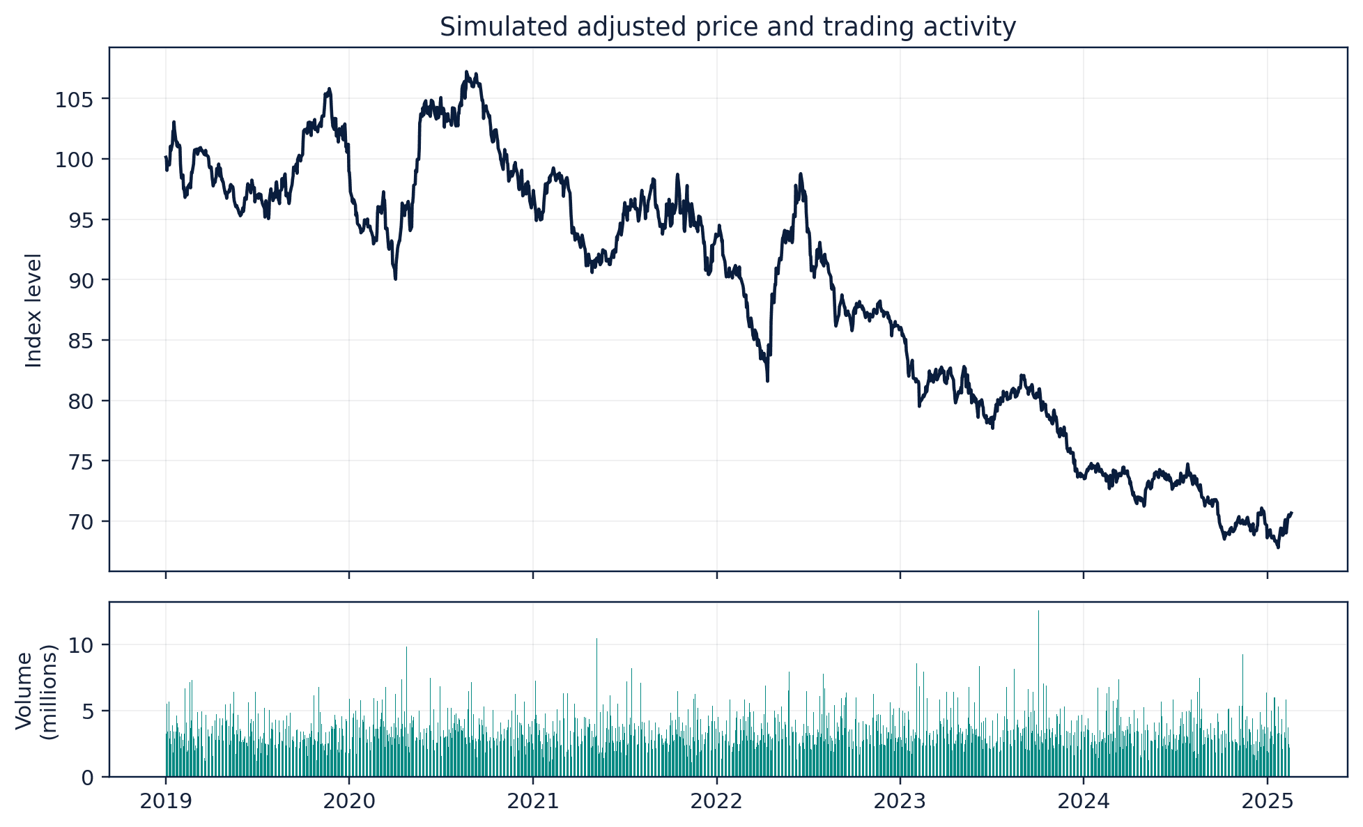
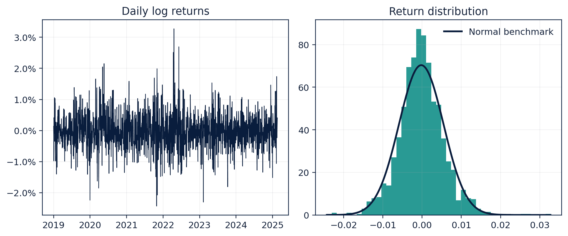
Visual evidence
36.8
Reference table
Why This Matters
Time-series transformations determine what a model is trying to explain or forecast.
Common Mistake
Averaging daily returns to obtain a monthly return. Compounding or summing log returns is the coherent aggregation.
Ceteris LAB Tip
Write the frequency and transformation directly in the variable name or metadata, such as cpi_yoy_pct.
R-to-Python / Source Bridge
The first financial time-series lecture introduced prices, returns, exchange rates, interest rates, earnings, claims, and transactions. This chapter modernizes those examples with pandas time indexes and explicit aggregation (Tsay 2013).
| Quantity | Formula or rule | Aggregation |
|---|---|---|
| price level | P_t | last or average, depending question |
| simple return | P_t/P_{t-1}-1 | compound geometrically |
| log return | log(P_t)-log(P_{t-1}) | sum |
| volume | count or quantity | sum |
| rate | percentage level | average or period end |
Visual evidence
Additional Python demonstrations
Live Python
Source demonstration 2
Source demonstration 2
Stdout
Run Python to see results here.
Status / stderr
Ready to run Python in your browser.
Line-by-line guide
- Line 1Load a Python library needed for data work or regression.
- Line 3Create or update a Python object used in the analysis.
- Line 4Create or update a Python object used in the analysis.
- Line 5Create or update a Python object used in the analysis.
- Line 6Display a result so students can inspect the output.
Verified source output
[0.02, -0.0098, 0.0297]
[0.0198, -0.0099, 0.0293]
rate  volume
2026-01-31    30    3100
2026-02-28    58    2800
2026-03-31    59     100
[0.02, -0.0098, 0.0297] [0.0198, -0.0099, 0.0293]
rate volume 2026-01-31 30 3100 2026-02-28 58 2800 2026-03-31 59 100
Interpretation. The two measures are close for small changes but are not numerically identical.
Interpretation. The rate uses the last observation while volume is summed, reflecting different measurement concepts.
Guided practice
- 1Re-run Demonstration 17.1 and change one input while keeping the analytical question fixed.
- 2Explain in two sentences how the output supports, or fails to support, the chapter opening question.
- 3Add one validation check that would prevent a plausible error.
Exercises
- 1Calculate simple and log returns for a price series.
- 2Verify that summed log returns equal the total log return.
- 3Resample daily volume to monthly totals.
- 4Explain how a missing trading day differs from a missing quote.
Source and downloads
Chapter 36 of Fundamentals of Python for Financial Econometrics by Mohammad Safavi, Ph.D.. The lesson is an original Ceteris Lab web adaptation of the supplied publication package.
Live Python
Introduction to Time-Series Data: live Python
Introduction to Time-Series Data: live Python
Stdout
Run Python to see results here.
Status / stderr
Ready to run Python in your browser.
Line-by-line guide
- Line 1Load a Python library needed for data work or regression.
- Line 2Load a Python library needed for data work or regression.
- Line 4Create or update a Python object used in the analysis.
- Line 5Create or update a Python object used in the analysis.
- Line 6Create a log version of the variable so coefficients can be read approximately as percentages.
- Line 7Keep rows that have the variables required for this model.
- Line 8Keep rows that have the variables required for this model.
Python walkthrough
- 1`import numpy as np`: Loads a package or function used by the analysis.
- 2`import pandas as pd`: Loads a package or function used by the analysis.
- 3`prices = pd.Series([100, 102, 101, 104], index=pd.date_range("2026-01-01", periods=4, freq="`: Creates or updates a named object used by later steps.
- 4`simple = prices.pct_change()`: Creates or updates a named object used by later steps.
- 5`log_return = np.log(prices).diff()`: Creates or updates a named object used by later steps.
- 6`print(simple.dropna().round(4).tolist())`: Displays a result so it can be checked and interpreted.
- 7`print(log_return.dropna().round(4).tolist())`: Displays a result so it can be checked and interpreted.
Live notebook
Run this lesson as a notebook
Open an editable notebook cell-by-cell, run Python in the browser, and download the `.ipynb` file for later.
Related dataset
Ceteris Lab teaching sample
Estimated time
25 to 40 min
Packages
pandas, numpy
Expected output
Printed Python results that can be compared with the lesson explanation.
Learning goals
- Load and inspect Ceteris Lab teaching sample.
- Run the Python cells connected to Introduction to Time-Series Data.
- Interpret the output using Create and validate time indexes and levels, changes, growth rates, and returns.
Common errors
- File not found: check that wage_sample.csv is installed or use the course data folder.
- Package import error: use the browser notebook first, then download for local Jupyter if your local packages differ.
- Column name error: compare your variable names with the dataset variables listed for this notebook.
Dataset path helper
import pandas as pd

df = pd.read_csv("/data/wage_sample.csv")
df.head()
Interactive activity
Chapter 36 interactive
Assumption stress test
What should determine the strength of an econometric claim?
Immediate feedback
Choose a decision, then test how the claim changes as evidence becomes stronger or weaker.
Try it yourself
Write one plain-English sentence explaining the main idea from this lesson.
Common mistakes
Check these before you move on.
Return to the lesson assumptions, units, diagnostics, and source evidence to replace this shortcut with a defensible interpretation.
Quick quiz
Which statement best answers the Chapter 36 opening question: What changes when observations are ordered in time and yesterday can influence today?
Quick quiz
Which practice should be avoided when applying Introduction to Time-Series Data?
Quick quiz
What is the most defensible way to interpret the Python demonstration?
Quick quiz
Why does Chapter 36 matter in an applied econometrics workflow?
Key takeaway
Time order and frequency are analytical structure. Levels, changes, simple returns, and log returns serve different purposes. Aggregation rules depend on whether a variable is a stock, flow, rate, or return.