Lesson 13
Descriptive Statistics and Exploratory Data Analysis
Big question
How can a dataset be summarized without letting one number erase its shape?
Lesson progress
Complete checkpoints as you learn
Learning objectives
- Calculate location, spread, shape, and dependence statistics.
- Compare conventional and robust summaries.
- Interpret skewness and kurtosis.
- Use plots and tables together.
- Prerequisites: Chapters 9 to 12.
- Key terms: mean, median, variance, skewness, kurtosis, correlation.
Simple explanation
The mean balances all observations and is sensitive to extreme values. The median identifies the middle and is more robust. Variance and standard deviation describe dispersion around the mean, while the interquartile range describes the middle half of the data. These measures should be selected according to the distribution and the decision, not reported mechanically.
Key terms
- Calculate location, spread, shape, and dependence statistics
- A core idea in Chapter 13 that students apply carefully in economic analysis.
- Compare conventional and robust summaries
- A core idea in Chapter 13 that students apply carefully in economic analysis.
- skewness and kurtosis
- A core idea in Chapter 13 that students apply carefully in economic analysis.
- plots and tables together
- A core idea in Chapter 13 that students apply carefully in economic analysis.
- Prerequisites: Chapters 9 to 12
- A core idea in Chapter 13 that students apply carefully in economic analysis.
- Key terms: mean, median, variance, skewness, kurtosis, correlation
- A core idea in Chapter 13 that students apply carefully in economic analysis.
Analytical workflow
Interpret the expression in words and units before using it in a claim.
Example
Interpretation. The extreme value pulls the mean and standard deviation upward, while the median and IQR remain close to the central cluster.
Prerequisites
- Complete the preceding course chapters or review their summaries as needed.
Full theory and examples
13.2
Location and spread answer different questions
The mean balances all observations and is sensitive to extreme values. The median identifies the middle and is more robust. Variance and standard deviation describe dispersion around the mean, while the interquartile range describes the middle half of the data. These measures should be selected according to the distribution and the decision, not reported mechanically.
13.3
Shape matters in finance
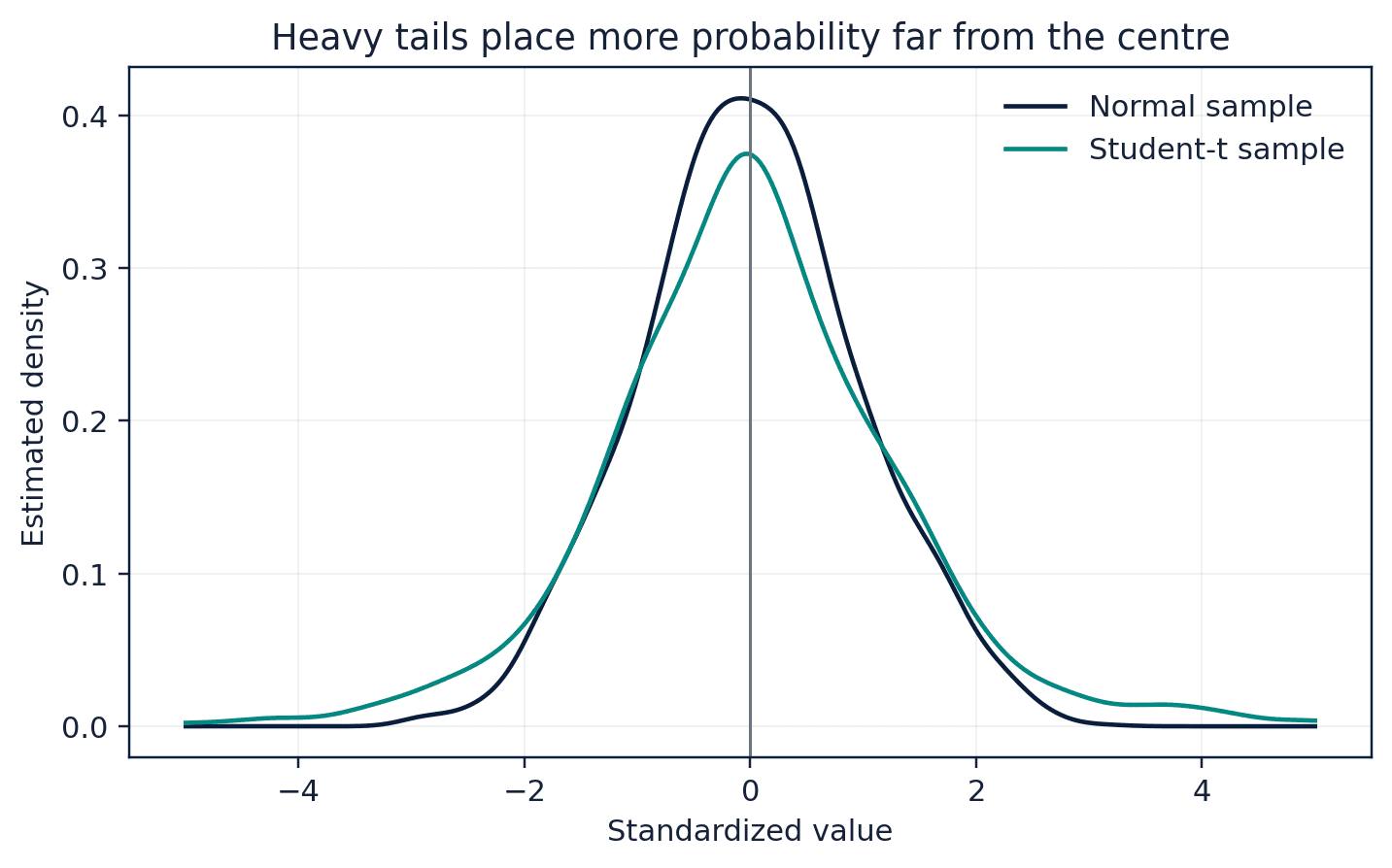
Asset returns often exhibit skewness and heavier tails than a Gaussian model. Skewness describes asymmetry; kurtosis describes the weight of tails and concentration relative to a reference convention. Software differs on whether reported kurtosis subtracts three. The book uses Fisher excess kurtosis when the normal reference is zero and labels the convention explicitly (Tsay 2010).
13.4
Dependence is not a single coefficient
Pearson correlation measures linear association and can be dominated by outliers. Spearman and Kendall correlations use ranks and capture monotonic relationships. None proves causality, and correlation can vary across regimes or frequencies. Exploratory analysis should combine scatterplots, subgroup summaries, and time ordering before a dependence measure is interpreted.
13.5
Core equations
Sample variance
The denominator n-1 estimates population variance under standard independent-sampling assumptions.
13.6
Python demonstrations
13.6.1
Demonstration 13.1: Conventional and robust summaries
Verified output
Interpretation. The extreme value pulls the mean and standard deviation upward, while the median and IQR remain close to the central cluster.
13.6.2
Demonstration 13.2: Distribution shape
Verified output
Interpretation. The excess kurtosis is well above zero, consistent with heavier tails than a normal distribution.
13.7
Visual evidence
13.8
Reference table
Why This Matters
Exploration reveals which summaries, transformations, and models are plausible before formal estimation begins.
Common Mistake
Reporting correlation to three decimals without showing the scatterplot, subgroup structure, or time ordering.
Ceteris LAB Tip
Pair every important summary statistic with a plot that can reveal why it takes that value.
R-to-Python / Source Bridge
The source lecture on financial time series emphasized skewness, heavy tails, and dependence. This chapter preserves those foundations and adds explicit convention checks and robust alternatives (Tsay 2013).
| Statistic | Sensitive to extremes? | Primary meaning |
|---|---|---|
| mean | Yes | arithmetic centre |
| median | Less | middle observation |
| standard deviation | Yes | dispersion around mean |
| IQR | Less | middle-half spread |
| skewness | Yes | asymmetry |
| excess kurtosis | Very | tail weight and peakedness |
Visual evidence
Additional Python demonstrations
Live Python
Source demonstration 2
Source demonstration 2
Stdout
Run Python to see results here.
Status / stderr
Ready to run Python in your browser.
Line-by-line guide
- Line 1Load a Python library needed for data work or regression.
- Line 2Load a Python library needed for data work or regression.
- Line 4Create or update a Python object used in the analysis.
- Line 5Create or update a Python object used in the analysis.
- Line 6Display a result so students can inspect the output.
- Line 7Display a result so students can inspect the output.
Verified source output
{'mean': np.float64(20.2), 'median': np.float64(12.0), 'std': np.float64(19.485892332659542), 'iqr': np.float64(2.0)}0.302 10.268
0.302
10.268
import pandas as pd
from scipy import stats
x = pd.Series([10, 11, 12, 13, 55])
print({
"mean": x.mean(),
"median": x.median(),
Interpretation. The extreme value pulls the mean and standard deviation upward, while the median and IQR remain close to the central cluster.
Interpretation. The excess kurtosis is well above zero, consistent with heavier tails than a normal distribution.
Guided practice
- 1Re-run Demonstration 13.1 and change one input while keeping the analytical question fixed.
- 2Explain in two sentences how the output supports, or fails to support, the chapter opening question.
- 3Add one validation check that would prevent a plausible error.
Exercises
- 1Compare mean and median in a skewed sample.
- 2Calculate Fisher and Pearson kurtosis and explain the difference.
- 3Compare Pearson and Spearman correlations.
- 4Build a grouped descriptive-statistics table.
Source and downloads
Chapter 13 of Fundamentals of Python for Financial Econometrics by Mohammad Safavi, Ph.D.. The lesson is an original Ceteris Lab web adaptation of the supplied publication package.
Live Python
Descriptive Statistics and Exploratory Data Analysis: live Python
Descriptive Statistics and Exploratory Data Analysis: live Python
Stdout
Run Python to see results here.
Status / stderr
Ready to run Python in your browser.
Line-by-line guide
- Line 1Load a Python library needed for data work or regression.
- Line 2Load a Python library needed for data work or regression.
- Line 4Create or update a Python object used in the analysis.
- Line 5Display a result so students can inspect the output.
- Line 6Run this Python instruction as part of the lesson workflow.
- Line 7Run this Python instruction as part of the lesson workflow.
- Line 8Run this Python instruction as part of the lesson workflow.
- Line 9Run this Python instruction as part of the lesson workflow.
- Line 10Run this Python instruction as part of the lesson workflow.
Python walkthrough
- 1`import pandas as pd`: Loads a package or function used by the analysis.
- 2`from scipy import stats`: Loads a package or function used by the analysis.
- 3`x = pd.Series([10, 11, 12, 13, 55])`: Creates or updates a named object used by later steps.
- 4`print({`: Displays a result so it can be checked and interpreted.
- 5`"mean": x.mean(),`: Executes the next transparent step in the workflow.
- 6`"median": x.median(),`: Executes the next transparent step in the workflow.
- 7`"std": x.std(),`: Executes the next transparent step in the workflow.
- 8`"iqr": stats.iqr(x),`: Executes the next transparent step in the workflow.
- 9`})`: Executes the next transparent step in the workflow.
Live notebook
Run this lesson as a notebook
Open an editable notebook cell-by-cell, run Python in the browser, and download the `.ipynb` file for later.
Related dataset
Ceteris Lab teaching sample
Estimated time
15 to 25 min
Packages
pandas, numpy, matplotlib
Expected output
A printed summary plus a chart in the output panel.
Learning goals
- Load and inspect Ceteris Lab teaching sample.
- Run the Python cells connected to Descriptive Statistics and Exploratory Data Analysis.
- Interpret the output using Calculate location, spread, shape, and dependence statistics and Compare conventional and robust summaries.
Common errors
- File not found: check that wage_sample.csv is installed or use the course data folder.
- Package import error: use the browser notebook first, then download for local Jupyter if your local packages differ.
- Column name error: compare your variable names with the dataset variables listed for this notebook.
Dataset path helper
import pandas as pd

df = pd.read_csv("/data/wage_sample.csv")
df.head()
Interactive activity
Chapter 13 interactive
Data evidence planner
Which choice makes an exploratory result easier to defend?
Immediate feedback
Choose a decision, then test how the claim changes as evidence becomes stronger or weaker.
Try it yourself
Write one plain-English sentence explaining the main idea from this lesson.
Common mistakes
Check these before you move on.
Return to the lesson assumptions, units, diagnostics, and source evidence to replace this shortcut with a defensible interpretation.
Quick quiz
Which statement best answers the Chapter 13 opening question: How can a dataset be summarized without letting one number erase its shape?
Quick quiz
Which practice should be avoided when applying Descriptive Statistics and Exploratory Data Analysis?
Quick quiz
What is the most defensible way to interpret the Python demonstration?
Quick quiz
Why does Chapter 13 matter in an applied econometrics workflow?
Key takeaway
Location, spread, shape, and dependence describe different features. Robust statistics reduce sensitivity to extremes. Financial returns frequently require heavy-tail diagnostics.