Lesson 38
AR, MA, ARMA, ARIMA, and Forecasting
Big question
How can past values and past shocks be organized into a model that produces honest forecasts and uncertainty?
Lesson progress
Complete checkpoints as you learn
Learning objectives
- Interpret AR and MA dynamics.
- Use ACF, PACF, AIC, and BIC for model guidance.
- Estimate ARIMA models with statsmodels.
- Evaluate point and interval forecasts out of sample.
- Prerequisites: Chapter 18.
- Key terms: AR, MA, ARMA, ARIMA, AIC, forecast interval.
Simple explanation
An AR model expresses the current value as a linear function of past values and a new shock. In a stationary AR(1), the coefficient controls persistence and the speed of mean reversion. Values near one produce slow decay; negative values produce alternating adjustment. Higher-order AR models can represent richer cycles but also create unstable roots if selected without care.
Key terms
- AR and MA dynamics
- A core idea in Chapter 38 that students apply carefully in economic analysis.
- ACF, PACF, AIC, and BIC for model guidance
- A core idea in Chapter 38 that students apply carefully in economic analysis.
- Estimate ARIMA models with statsmodels
- A core idea in Chapter 38 that students apply carefully in economic analysis.
- Evaluate point and interval forecasts out of sample
- A core idea in Chapter 38 that students apply carefully in economic analysis.
- Prerequisites: Chapter 18
- A core idea in Chapter 38 that students apply carefully in economic analysis.
- Key terms: AR, MA, ARMA, ARIMA, AIC, forecast interval
- A core idea in Chapter 38 that students apply carefully in economic analysis.
Analytical workflow
Interpret the expression in words and units before using it in a claim.
Example
Interpretation. The estimates recover the simulated AR and MA structure approximately. Sampling variation and likelihood conventions prevent exact equality.
Prerequisites
- Complete the preceding course chapters or review their summaries as needed.
Full theory and examples
38.2
Autoregression describes persistence
An AR model expresses the current value as a linear function of past values and a new shock. In a stationary AR(1), the coefficient controls persistence and the speed of mean reversion. Values near one produce slow decay; negative values produce alternating adjustment. Higher-order AR models can represent richer cycles but also create unstable roots if selected without care.
38.3
Moving averages describe shock memory
An MA model expresses the current observation as a combination of current and past innovations. Innovations are not observed directly and are recovered during estimation. Invertibility allows the model to be represented in terms of observed history. Software conventions differ in the sign assigned to MA coefficients, so equations and package parameterization must be checked before comparing R and Python output.
38.4
Forecasting is an evaluation design
ARIMA combines autoregressive, differencing, and moving-average components. AIC and BIC compare likelihood with complexity penalties, but the lowest in-sample criterion is not guaranteed to forecast best. A credible evaluation reserves later observations, fits only on available history, produces point and interval forecasts, and reports metrics such as MAE or RMSE alongside a naive benchmark. Rolling-origin evaluation better reflects repeated forecasting than one lucky split.
38.5
Core equations
AR(1)
The stationary process reverts toward mean mu at a rate controlled by phi.
Half-life
For 0<|phi|<1, h is the approximate number of periods required for a deviation to halve.
38.6
Python demonstrations
38.6.1
Demonstration 19.1: Simulate and fit an ARMA process
Verified output
Interpretation. The estimates recover the simulated AR and MA structure approximately. Sampling variation and likelihood conventions prevent exact equality.
38.6.2
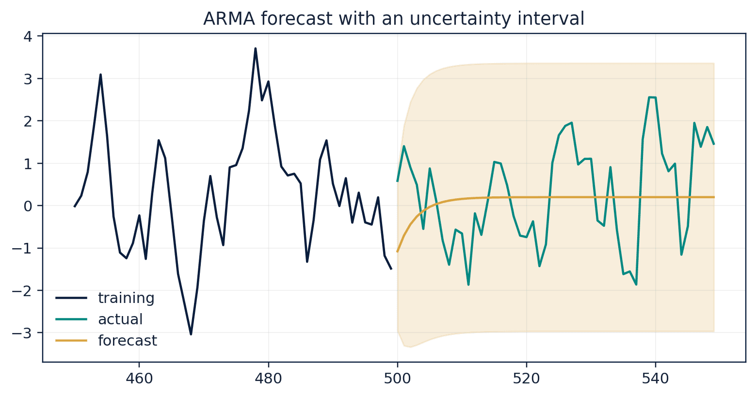
Demonstration 19.2: Forecast with an interval
Verified output
Interpretation. The forecast returns toward the estimated mean while uncertainty expands with horizon.
38.7
Visual evidence
38.8
Reference table
Why This Matters
Forecast models are useful only when their information set, benchmark, horizon, and evaluation window match the decision.
Common Mistake
Selecting p and q solely by scanning many specifications on the full sample, then reporting the best fit as an out-of-sample success.
Ceteris LAB Tip
Always compare an ARIMA forecast with a simple benchmark such as the historical mean, last value, or seasonal naive forecast.
R-to-Python / Source Bridge
The source AR lecture develops mean reversion, forecast-error variance, half-life, AIC/BIC, and Ljung-Box checks. The Python implementation uses statsmodels and explicitly documents intercept and MA-sign conventions (Tsay 2013).
| Pattern | AR suggestion | MA suggestion |
|---|---|---|
| ACF tails off; PACF cuts off | AR(p) | not primary |
| ACF cuts off; PACF tails off | not primary | MA(q) |
| both tail off | ARMA candidate | ARMA candidate |
| slow decay in levels | possible unit root | difference before ARMA |
Visual evidence
Additional Python demonstrations
Live Python
Source demonstration 2
Source demonstration 2
Stdout
Run Python to see results here.
Status / stderr
Ready to run Python in your browser.
Line-by-line guide
- Line 1Create or update a Python object used in the analysis.
- Line 2Create or update a Python object used in the analysis.
- Line 3Create or update a Python object used in the analysis.
- Line 4Display a result so students can inspect the output.
- Line 5Display a result so students can inspect the output.
Verified source output
[-0.055 0.619 0.394 0.932]
[-0.603 -0.394 -0.265 -0.185 -0.136]
[-2.495  1.29 ]
[-0.055 0.619 0.394 0.932]
[-0.603 -0.394 -0.265 -0.185 -0.136] [-2.495 1.29 ]
Interpretation. The estimates recover the simulated AR and MA structure approximately. Sampling variation and likelihood conventions prevent exact equality.
Interpretation. The forecast returns toward the estimated mean while uncertainty expands with horizon.
Guided practice
- 1Re-run Demonstration 19.1 and change one input while keeping the analytical question fixed.
- 2Explain in two sentences how the output supports, or fails to support, the chapter opening question.
- 3Add one validation check that would prevent a plausible error.
Exercises
- 1Simulate an AR(1) with phi 0.8 and calculate its half-life.
- 2Fit ARIMA candidates and compare AIC and BIC.
- 3Reserve the last 20 observations for evaluation.
- 4Explain why forecast intervals widen with horizon.
Source and downloads
Chapter 38 of Fundamentals of Python for Financial Econometrics by Mohammad Safavi, Ph.D.. The lesson is an original Ceteris Lab web adaptation of the supplied publication package.
Live Python
AR, MA, ARMA, ARIMA, and Forecasting: live Python
AR, MA, ARMA, ARIMA, and Forecasting: live Python
Stdout
Run Python to see results here.
Status / stderr
Ready to run Python in your browser.
Line-by-line guide
- Line 1Load a Python library needed for data work or regression.
- Line 2Load a Python library needed for data work or regression.
- Line 3Load a Python library needed for data work or regression.
- Line 5Create or update a Python object used in the analysis.
- Line 6Create or update a Python object used in the analysis.
- Line 7Create or update a Python object used in the analysis.
- Line 8Create or update a Python object used in the analysis.
- Line 9Display a result so students can inspect the output.
Python walkthrough
- 1`import numpy as np`: Loads a package or function used by the analysis.
- 2`from statsmodels.tsa.arima_process import ArmaProcess`: Loads a package or function used by the analysis.
- 3`from statsmodels.tsa.arima.model import ARIMA`: Loads a package or function used by the analysis.
- 4`rng = np.random.default_rng(19)`: Creates or updates a named object used by later steps.
- 5`process = ArmaProcess(ar=[1, -0.65], ma=[1, 0.35])`: Creates or updates a named object used by later steps.
- 6`x = process.generate_sample(500, distrvs=rng.standard_normal)`: Creates or updates a named object used by later steps.
- 7`fit = ARIMA(x, order=(1, 0, 1), trend="c").fit()`: Fits the specified statistical or machine-learning model.
- 8`print(fit.params.round(3))`: Displays a result so it can be checked and interpreted.
Live notebook
Run this lesson as a notebook
Open an editable notebook cell-by-cell, run Python in the browser, and download the `.ipynb` file for later.
Related dataset
Ceteris Lab teaching sample
Estimated time
25 to 40 min
Packages
pandas, numpy, statsmodels, patsy
Expected output
Printed Python results that can be compared with the lesson explanation.
Learning goals
- Load and inspect Ceteris Lab teaching sample.
- Run the Python cells connected to AR, MA, ARMA, ARIMA, and Forecasting.
- Interpret the output using AR and MA dynamics and ACF, PACF, AIC, and BIC for model guidance.
Common errors
- File not found: check that wage_sample.csv is installed or use the course data folder.
- Package import error: use the browser notebook first, then download for local Jupyter if your local packages differ.
- Column name error: compare your variable names with the dataset variables listed for this notebook.
Dataset path helper
import pandas as pd

df = pd.read_csv("/data/wage_sample.csv")
df.head()
Interactive activity
Chapter 38 interactive
Assumption stress test
What should determine the strength of an econometric claim?
Immediate feedback
Choose a decision, then test how the claim changes as evidence becomes stronger or weaker.
Try it yourself
Write one plain-English sentence explaining the main idea from this lesson.
Common mistakes
Check these before you move on.
Return to the lesson assumptions, units, diagnostics, and source evidence to replace this shortcut with a defensible interpretation.
Quick quiz
Which statement best answers the Chapter 38 opening question: How can past values and past shocks be organized into a model that produces honest forecasts and uncertainty?
Quick quiz
Which practice should be avoided when applying AR, MA, ARMA, ARIMA, and Forecasting?
Quick quiz
What is the most defensible way to interpret the Python demonstration?
Quick quiz
Why does Chapter 38 matter in an applied econometrics workflow?
Key takeaway
AR models encode persistence; MA models encode shock memory. ARIMA adds differencing for integrated series. Model selection must be followed by residual diagnostics and genuine out-of-sample evaluation.